Matplotlib 第五课

1. part-IV, Limits, Legends, and Layouts
- 1.1. Artists
  - 1.1.1. Primative Artists
  - 1.1.2. Container Artists
- 1.2. Collections

1 part-IV, Limits, Legends, and Layouts

from __future__ import print_function
import matplotlib
import numpy as np
import matplotlib.pyplot as plt

1.1 Artists

Anything can draw or can be draw is an Artist.

Figure Artist.
Axes Artist.
plot Artist.
bar Artist.
scatter Artist.
etc.

There are two main classes of Artists: primatives and containers. Below is a sample of these primitives.

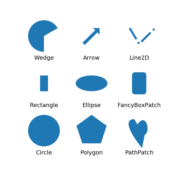
1.1.1 Primative Artists

primitives Artist:

wedge artist
arrow artist
line2D artist
rectangle artist
ellipse artist
fancyBoxPatch artist
etc

from matplotlib.collections import PatchCollection
import matplotlib.path as mpath
import matplotlib.patches as mpatches
import matplotlib.lines as mlines

fig, ax = plt.subplots(1, 1, figsize=(7,7))

# create 3x3 grid to plot the artists
pos = np.mgrid[0.2:0.8:3j, 0.2:0.8:3j].reshape(2, -1) # <- '-1' means I don't care, you compute it for me.
patches = []

# add a circle
art = mpatches.Circle(pos[:, 0], 0.1, ec="none")
patches.append(art)
plt.text(pos[0, 0], pos[1, 0] - 0.15, "Circle", ha="center", size=14)

# add a rectangle
art = mpatches.Rectangle(pos[:, 1] - [0.025, 0.05], 0.05, 0.1, ec="none")
patches.append(art)
plt.text(pos[0, 1], pos[1, 1] - 0.15, "Rectangle", ha="center", size=14)

# add a wedge
wedge = mpatches.Wedge(pos[:, 2], 0.1, 30, 270, ec="none")
patches.append(wedge)
plt.text(pos[0, 2], pos[1, 2] - 0.15, "Wedge", ha="center", size=14)

# add a Polygon
polygon = mpatches.RegularPolygon(pos[:, 3], 5, 0.1)
patches.append(polygon)
plt.text(pos[0, 3], pos[1, 3] - 0.15, "Polygon", ha="center", size=14)

#add an ellipse
ellipse = mpatches.Ellipse(pos[:, 4], 0.2, 0.1)
patches.append(ellipse)
plt.text(pos[0, 4], pos[1, 4] - 0.15, "Ellipse", ha="center", size=14)

#add an arrow
arrow = mpatches.Arrow(pos[0, 5] - 0.05, pos[1, 5] - 0.05, 0.1, 0.1, width=0.1)
patches.append(arrow)
plt.text(pos[0, 5], pos[1, 5] - 0.15, "Arrow", ha="center", size=14)

# add a path patch
Path = mpath.Path
verts = np.array([
     (0.158, -0.257),
     (0.035, -0.11),
     (-0.175, 0.20),
     (0.0375, 0.20),
     (0.085, 0.115),
     (0.22, 0.32),
     (0.3, 0.005),
     (0.20, -0.05),
     (0.158, -0.257),
    ])
verts = verts - verts.mean(0)
codes = [Path.MOVETO,
         Path.CURVE4, Path.CURVE4, Path.CURVE4, Path.LINETO,
         Path.CURVE4, Path.CURVE4, Path.CURVE4, Path.CLOSEPOLY]

path = mpath.Path(verts / 2.5 + pos[:, 6], codes)
patch = mpatches.PathPatch(path)
patches.append(patch)
plt.text(pos[0, 6], pos[1, 6] - 0.15, "PathPatch", ha="center", size=14)

# add a fancy box
fancybox = mpatches.FancyBboxPatch(
        pos[:, 7] - [0.025, 0.05], 0.05, 0.1,
        boxstyle=mpatches.BoxStyle("Round", pad=0.02))
patches.append(fancybox)
plt.text(pos[0, 7], pos[1, 7] - 0.15, "FancyBoxPatch", ha="center", size=14)

# add a line
x,y = np.array([[-0.06, 0.0, 0.1], [0.05,-0.05, 0.05]])
line = mlines.Line2D(x+pos[0, 8], y+pos[1, 8], lw=5.)
plt.text(pos[0, 8], pos[1, 8] - 0.15, "Line2D", ha="center", size=14)

collection = PatchCollection(patches)
ax.add_collection(collection)
ax.add_line(line)
ax.set_axis_off()

plt.show()

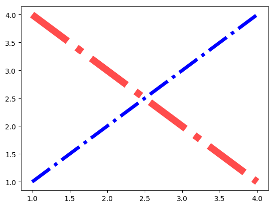
1.1.2 Container Artists

Containers are objects like Figure and Axes. Containers are given primitives to draw. The plotting functions we discussed back in Parts 1 & 2 are convenience functions that generate these primitives and places them into the appropriate containers. In fact, most of those functions will return artist objects (or a list of artist objects) as well as store them into the appropriate axes container.

As discussed in Part 3, there is a wide range of properties that can be defined for your plots. These properties are processed and applied to their primitives. Ultimately, you can override anything you want just by directly setting a property to the object itself.

fig, ax = plt.subplots(1, 1)
lines = plt.plot([1, 2, 3, 4], [1, 2, 3, 4], 'b', [1, 2, 3, 4], [4, 3, 2, 1], 'r')
lines[0].set(linewidth=5)
lines[1].set(linewidth=10, alpha=0.7)
plt.show()

To see what properties are set for an artist, use getp()

fig = plt.figure()
print(plt.getp(fig.patch))
plt.close(fig)

1.2 Collections

Collections In addition to the Figure and Axes containers, there is another special type of container called a Collection. A Collection usually contains a list of primitives of the same kind that should all be treated similiarly. For example, a CircleCollection would have a list of Circle objects all with the same color, size, and edge width. Individual property values for artists in the collection can also be set (in some cases).

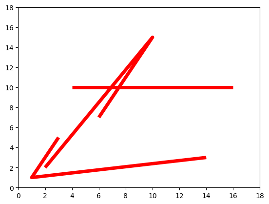
1.2.1 do settings to all items of collection

.           do settings to all items
.                     |
.                     v
.   3 lines ---> collections --->  ---> axes ---> show()

from matplotlib.collections import LineCollection
fig, ax = plt.subplots(1, 1)                       # <- create figure and axes
# A collection of 3 lines
lc = LineCollection([[(4, 10), (16, 10)],          # <- create a collection of 3lines
                     [(2, 2), (10, 15), (6, 7)],
                     [(14, 3), (1, 1), (3, 5)]])
lc.set_color('r')                                  # <- do some settings to all lines
lc.set_linewidth(5)                                #    inside of this collection
ax.add_collection(lc)                              # <- add this collection to axes created above
ax.set_xlim(0, 18)
ax.set_ylim(0, 18)
plt.show()

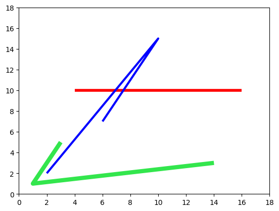
1.2.2 do settings to separate items of collection

# Now set individual properties in a collection
fig, ax = plt.subplots(1, 1)
lc = LineCollection([[(4, 10), (16, 10)],
                     [(2, 2), (10, 15), (6, 7)],
                     [(14, 3), (1, 1), (3, 5)]])
lc.set_color(['r', 'blue', (0.2, 0.9, 0.3)]) # <- do separate settings in an array
lc.set_linewidth([4, 3, 6])                  # <- do separate settings in an array
ax.add_collection(lc)                        # <- add collection to axes
ax.set_xlim(0, 18)
ax.set_ylim(0, 18)
plt.show()

1.2.3 more specified collection

There are other kinds of collections that are not just simply a list of primitives, but are Artists in their own right. These special kinds of collections take advantage of various optimizations that can be assumed when rendering similar or identical things. You use these collections all the time whether you realize it or not! Markers are implemented this way (so, whenever you do plot() or scatter(), for example).

eg:

RegularPolyCollection class
StarPolygonCollection class

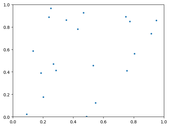
1.2.4 RegularPolyCollection

from matplotlib.collections import RegularPolyCollection

fig, ax = plt.subplots(1, 1)
offsets = np.random.rand(20, 2)       # <- produce the 2-D location of 20 polygon
collection = RegularPolyCollection(   # <- create a RegularPolyCollection
    numsides=5,                       # <- all polygon have 5 sides
    sizes=(15,),                      # <- give each column of polygon the size,
                                      #    for 2D collection:(x,y), for 3D collection:(x,y,z)
    offsets=offsets,                  # <- give location of all polygon
    transOffset=ax.transData,
    )
ax.add_collection(collection)
plt.show()

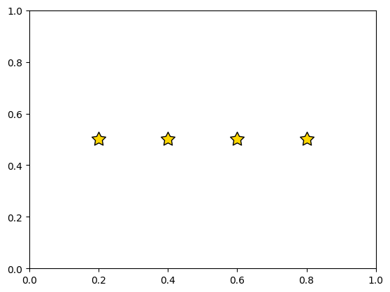
1.2.5 StarPolygonCollection

from matplotlib.collections import StarPolygonCollection

fig, ax = plt.subplots(1,1)

offsets = zip([0.2,0.4,0.6,0.8], [0.5]*4)
offsets = [[i,j] for i,j in offsets]

collection = StarPolygonCollection(
    5,                         # <- all StartPolygons have 5 angles
    offsets=offsets,           # <- all location of each StartPolygon
    transOffset=ax.transData,
    facecolors=['gold'],       # <- facecolors, you can give each a color
    sizes=[175],
    edgecolors=['k']           # <- edgecolors, you can give each a color
)
ax.add_collection(collection)
plt.show()