Matplotlib 第六课

1. part-VI, mpl_toolkits
- 1.1. mpl_tookits.mplot3d
- 1.2. mpl_toolkits.axes_grid1

import matplotlib
import numpy as np
import matplotlib.pyplot as plt

1 part-VI, mpl_toolkits

In addition to the core library of Matplotlib, there are a few additional utilities that are set apart from Matplotlib proper for some reason or another, but are often shipped with Matplotlib.

Basemap - shipped separately from matplotlib due to size of mapping data that are included.
mplot3d - shipped with matplotlib to provide very simple, rudimentary 3D plots in the same style as matplotlib's 2D plots.
axes_grid1 - An enhanced SubplotAxes. Very Enhanced!

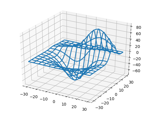
1.1 mpl_tookits.mplot3d

By taking advantage of Matplotlib's z-order layering engine, mplot3d emulates 3D plotting by projecting 3D data into 2D space, layer by layer. While it isn't going to replace any of the true 3D plotting libraries anytime soon, its goal is to allow for Matplotlib users to produce 3D plots with the same amount of simplicity as 2D plots.

from mpl_toolkits.mplot3d import Axes3D, axes3d

fig, ax = plt.subplots(1, 1, subplot_kw={'projection': '3d'})
X, Y, Z = axes3d.get_test_data(0.05)
ax.plot_wireframe(X, Y, Z, rstride=10, cstride=10)

plt.show()

1.2 mpl_toolkits.axes_grid1

This module was originally intended as a collection of helper classes to ease the displaying of (possibly multiple) images with Matplotlib. Some of the functionality has come to be useful for non-image plotting as well. Some classes deals with the sizing and positioning of multiple Axes relative to each other (ImageGrid, RGB Axes, and AxesDivider). The ParasiteAxes allow for the plotting of multiple datasets in the same axes, but with each their own x or y scale. Also, there is the AnchoredArtist that can be used to anchor particular artist objects in place.

One can get a sense of the neat things that can be done with this toolkit by browsing through its user guide linked above. There is one particular feature that is an absolute must-have for me – automatic allocation of space for colorbars.

See ImageGrid() here, they are used in similar manner.

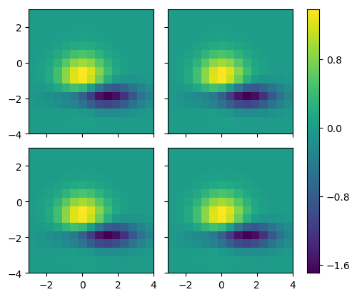
1.2.1 AxesGrid

from mpl_toolkits.axes_grid1 import AxesGrid
def get_demo_image():
    import numpy as np
    from matplotlib.cbook import get_sample_data
    f = get_sample_data("axes_grid/bivariate_normal.npy", asfileobj=False)
    z = np.load(f)
    # z is a numpy array of 15x15
    return z, (-3, 4, -4, 3)

fig = plt.figure()
grid = AxesGrid(fig, 111, # similar to subplot(111)
                nrows_ncols = (2, 2),
                axes_pad = 0.2,
                share_all=True,
                label_mode = "L",  # similar to "label_outer"
                cbar_location = "right",
                cbar_mode="single",
)

Z, extent = get_demo_image()  # demo image
for i in range(4):
    im = grid[i].imshow(Z, extent=extent, interpolation="nearest")

grid.cbar_axes[0].colorbar(im)
plt.show()

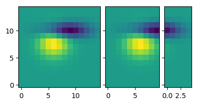
1.2.2 ImageGrid

See ImageGrid() here, more readable introduction.

import matplotlib.pyplot as plt
from mpl_toolkits.axes_grid1 import ImageGrid

def get_demo_image():
    import numpy as np
    from matplotlib.cbook import get_sample_data
    f = get_sample_data("axes_grid/bivariate_normal.npy", asfileobj=False)
    z = np.load(f)
    # z is a numpy array of 15x15
    return z, (-3, 4, -4, 3)

F = plt.figure(1, (4.5, 4.5))
grid = ImageGrid(F, 111,  # similar to subplot(111)
                 nrows_ncols=(1, 3),
                 axes_pad=0.1,
                 add_all=True,
                 label_mode="L",
)
Z, extent = get_demo_image()  # demo image

im1 = Z
im2 = Z[:, :10]
im3 = Z[:, 10:]
vmin, vmax = Z.min(), Z.max()
for i, im in enumerate([im1, im2, im3]):
    # print (i, im)
    ax = grid[i]
    # print ( "ax type: ")
    # print (type(ax) )
    ax.imshow(im, origin="lower", vmin=vmin,
              vmax=vmax, interpolation="nearest")

plt.draw()
plt.show()

1.2.3 Parasite Axes

寄生 Axes

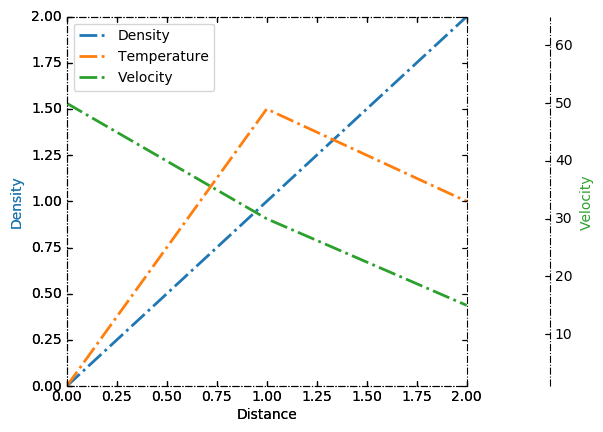
This next feature is commonly requested on the mailing lists. The problem is that most people who request it don't quite know how to describe it. We call it "Parasite Axes".

The ParasiteAxes allow for the plotting of multiple datasets in the same axes, but with each their own x or y scale.

"""
Parasite axis demo

The following code is an example of a parasite axis. It aims to show a user how
to plot multiple different values onto one single plot. Notice how in this
example, par1 and par2 are both calling twinx meaning both are tied directly to
the x-axis. From there, each of those two axis can behave separately from the
each other, meaning they can take on separate values from themselves as well as
the x-axis.
"""
from mpl_toolkits.axes_grid1 import host_subplot
import mpl_toolkits.axisartist as AA
import matplotlib.pyplot as plt

host = host_subplot(111, axes_class=AA.Axes)
plt.subplots_adjust(right=0.75)

par1 = host.twinx()
par2 = host.twinx()

offset = 60
new_fixed_axis = par2.get_grid_helper().new_fixed_axis
par2.axis["right"] = new_fixed_axis(loc="right",
                                    axes=par2,
                                    offset=(offset, 0))

par2.axis["right"].toggle(all=True)

host.set_xlim(0, 2)
host.set_ylim(0, 2)

host.set_xlabel("Distance")
host.set_ylabel("Density")
par1.set_ylabel("Temperature")
par2.set_ylabel("Velocity")

p1, = host.plot([0, 1, 2], [0, 1, 2], label="Density")
p2, = par1.plot([0, 1, 2], [0, 3, 2], label="Temperature")
p3, = par2.plot([0, 1, 2], [50, 30, 15], label="Velocity")

par1.set_ylim(0, 4)
par2.set_ylim(1, 65)

host.legend()

host.axis["left"].label.set_color(p1.get_color())
par1.axis["right"].label.set_color(p2.get_color())
par2.axis["right"].label.set_color(p3.get_color())

plt.show()

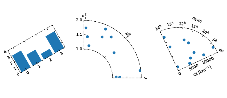
1.2.4 Floating Axes

And finally, as a nice teaser of what else axes_grid1 can do.

"""
Demo of the floating axes.

This demo shows features of functions in floating_axes:
    * Using scatter function and bar function with changing the
      shape of the plot.
    * Using GridHelperCurveLinear to rotate the plot and set the
      boundary of the plot.
    * Using FloatingSubplot to create a subplot using the return
      value from GridHelperCurveLinear.
    * Making sector plot by adding more features to GridHelperCurveLinear.
"""
from matplotlib.transforms import Affine2D
import mpl_toolkits.axisartist.floating_axes as floating_axes
import numpy as np
import mpl_toolkits.axisartist.angle_helper as angle_helper
from matplotlib.projections import PolarAxes
from mpl_toolkits.axisartist.grid_finder import (FixedLocator, MaxNLocator,
                                                 DictFormatter)
import matplotlib.pyplot as plt


def setup_axes1(fig, rect):
    """
    A simple one.
    """
    tr = Affine2D().scale(2, 1).rotate_deg(30)

    grid_helper = floating_axes.GridHelperCurveLinear(
        tr, extremes=(-0.5, 3.5, 0, 4))

    ax1 = floating_axes.FloatingSubplot(fig, rect, grid_helper=grid_helper)
    fig.add_subplot(ax1)

    aux_ax = ax1.get_aux_axes(tr)

    grid_helper.grid_finder.grid_locator1._nbins = 4
    grid_helper.grid_finder.grid_locator2._nbins = 4

    return ax1, aux_ax


def setup_axes2(fig, rect):
    """
    With custom locator and formatter.
    Note that the extreme values are swapped.
    """
    tr = PolarAxes.PolarTransform()

    pi = np.pi
    angle_ticks = [(0, r"$0$"),
                   (.25*pi, r"$\frac{1}{4}\pi$"),
                   (.5*pi, r"$\frac{1}{2}\pi$")]
    grid_locator1 = FixedLocator([v for v, s in angle_ticks])
    tick_formatter1 = DictFormatter(dict(angle_ticks))

    grid_locator2 = MaxNLocator(2)

    grid_helper = floating_axes.GridHelperCurveLinear(
        tr, extremes=(.5*pi, 0, 2, 1),
        grid_locator1=grid_locator1,
        grid_locator2=grid_locator2,
        tick_formatter1=tick_formatter1,
        tick_formatter2=None)

    ax1 = floating_axes.FloatingSubplot(fig, rect, grid_helper=grid_helper)
    fig.add_subplot(ax1)

    # create a parasite axes whose transData in RA, cz
    aux_ax = ax1.get_aux_axes(tr)

    aux_ax.patch = ax1.patch  # for aux_ax to have a clip path as in ax
    ax1.patch.zorder = 0.9  # but this has a side effect that the patch is
    # drawn twice, and possibly over some other
    # artists. So, we decrease the zorder a bit to
    # prevent this.

    return ax1, aux_ax


def setup_axes3(fig, rect):
    """
    Sometimes, things like axis_direction need to be adjusted.
    """

    # rotate a bit for better orientation
    tr_rotate = Affine2D().translate(-95, 0)

    # scale degree to radians
    tr_scale = Affine2D().scale(np.pi/180., 1.)

    tr = tr_rotate + tr_scale + PolarAxes.PolarTransform()

    grid_locator1 = angle_helper.LocatorHMS(4)
    tick_formatter1 = angle_helper.FormatterHMS()

    grid_locator2 = MaxNLocator(3)

    ra0, ra1 = 8.*15, 14.*15
    cz0, cz1 = 0, 14000
    grid_helper = floating_axes.GridHelperCurveLinear(
        tr, extremes=(ra0, ra1, cz0, cz1),
        grid_locator1=grid_locator1,
        grid_locator2=grid_locator2,
        tick_formatter1=tick_formatter1,
        tick_formatter2=None)

    ax1 = floating_axes.FloatingSubplot(fig, rect, grid_helper=grid_helper)
    fig.add_subplot(ax1)

    # adjust axis
    ax1.axis["left"].set_axis_direction("bottom")
    ax1.axis["right"].set_axis_direction("top")

    ax1.axis["bottom"].set_visible(False)
    ax1.axis["top"].set_axis_direction("bottom")
    ax1.axis["top"].toggle(ticklabels=True, label=True)
    ax1.axis["top"].major_ticklabels.set_axis_direction("top")
    ax1.axis["top"].label.set_axis_direction("top")

    ax1.axis["left"].label.set_text(r"cz [km$^{-1}$]")
    ax1.axis["top"].label.set_text(r"$\alpha_{1950}$")

    # create a parasite axes whose transData in RA, cz
    aux_ax = ax1.get_aux_axes(tr)

    aux_ax.patch = ax1.patch  # for aux_ax to have a clip path as in ax
    ax1.patch.zorder = 0.9  # but this has a side effect that the patch is
    # drawn twice, and possibly over some other
    # artists. So, we decrease the zorder a bit to
    # prevent this.

    return ax1, aux_ax


##########################################################
fig = plt.figure(figsize=(8, 4))
fig.subplots_adjust(wspace=0.3, left=0.05, right=0.95)

ax1, aux_ax1 = setup_axes1(fig, 131)
aux_ax1.bar([0, 1, 2, 3], [3, 2, 1, 3])

ax2, aux_ax2 = setup_axes2(fig, 132)
theta = np.random.rand(10)*.5*np.pi
radius = np.random.rand(10) + 1.
aux_ax2.scatter(theta, radius)

ax3, aux_ax3 = setup_axes3(fig, 133)

theta = (8 + np.random.rand(10)*(14 - 8))*15.  # in degrees
radius = np.random.rand(10)*14000.
aux_ax3.scatter(theta, radius)

plt.show()