Numpy-笔记2

1. Numpy
- 1.1. numpy io
- 1.2. numpy matrix operation

1 Numpy

1.1 numpy io

np.savetxt('path', nparrayRef, delimiter=',')
np.loadtxt('path', delimiter=',')

import os
import numpy as np
x = np.linspace(0, 2*np.pi, 4)
y = np.cos(x)

data = np.vstack((x,y))
data = data.T

# <- 'file i' in numpy.savetxt(filename, nparray)
np.savetxt('data.txt', data, delimiter=',')
print (os.path.abspath("data.txt"))

# <- 'file o'
z=np.loadtxt('data.txt', delimiter=',')

print (x)
print (y)
print (z)

1.2 numpy matrix operation

1.2.1 solve linear equation by numpy

np.linalg.inv(nparray)
np.linalg.solve(a,b) # <- solve ax=b
sym.linsolve

""" how to solve equation: ax=b
"""
import numpy as np
import sympy as sym

A = np.array([[3,2], [1,2]])
print (A)

b = np.array([1, 0])

# method-1: x = A^-1 * b
sol1 = np.dot(np.linalg.inv(A), b)
print (sol1)

# method-2: solve equation: ax=b by np.linalg.solve
sol2 = np.linalg.solve(A,b)
print (sol2)

# method-3: solve equation: ax=b by sympy.linsolve
sym.init_printing()
x, y = sym.symbols('x y')
z = sym.linsolve([3*x+2*y-1, x+2*y], (x, y))
sym.pprint(z)

1.2.2 solve nonlinear equation

from scipy.optimize import fsolve

def f(z):
    x=z[0]
    y=z[1]
    return [x+2*y, x**2+y**2-1]

z0 = [0,1]
z = fsolve(f,z0)
print (z)
print (f(z))

1.2.3 integration

from scipy.integrate import quad

def f(x):
    return x**2

# integrate from 0 to 2 on expression x^2
# method-1: using scipy
print (quad(f, 0, 2)[0])
print (2**3/3)

# method-2: using sympy
import sympy as sym
x = sym.Symbol('x')
f = sym.integrate(x**2, x)
f
# sym.pprint(f)

1.2.4 derivative

from scipy.misc import derivative

def f(x):
    return x**2

print (derivative(f, 2, dx=1e-10))

import sympy as sym
x=sym.Symbol('x')
f=sym.diff(x**3,x)
f
# f.subs(x, 2) #<- if x=2, what's the result of derivative

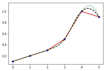
1.2.5 interpolation

from scipy.interpolate import interp1d
x = np.arange(0,6,1)
y = np.array([0.1,0.2,0.3,0.5,1.0,0.9])

%matplotlib inline
import matplotlib.pyplot as plt
plt.plot(x,y,'bo')

xp = np.linspace(0, 5, 100)

y1 = interp1d(x,y,kind='linear')
plt.plot(xp,y1(xp),'r-')

y2 = interp1d(x,y,kind='quadratic')
plt.plot(xp,y2(xp),'k--')

y3 = interp1d(x,y,kind='cubic')
plt.plot(xp,y3(xp),'g:')

[<matplotlib.lines.Line2D at 0x7fe196977630>]

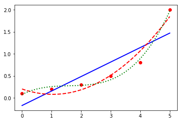
1.2.6 liear regression and a polynormial regression

a polynormial fit

import numpy as np
x = np.arange(0, 6, 1)
y = np.array([0.1, 0.2, 0.3,0.5, 0.8,2.0])

p1 = np.polyfit(x,y,1)
print (p1)
p2 = np.polyfit(x,y,2)
print (p2)
p3 = np.polyfit(x,y,3)
print (p3)

%matplotlib inline
import matplotlib.pyplot as plt

plt.plot(x,y,'ro')
xp = np.linspace(0, 5, 100)

plt.plot(xp,np.polyval(p1, xp),'b-', label='linear')
plt.plot(xp,np.polyval(p2, xp),'r--', label='quadratic')
plt.plot(xp,np.polyval(p3, xp),'g:', label='cubic')

plt.show()

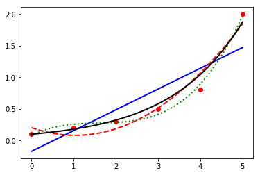
1.2.7 nonlinear regression

a curve fit

import numpy as np
from scipy.optimize import curve_fit

x = np.arange(0, 6, 1)
y = np.array([0.1, 0.2, 0.3,0.5, 0.8,2.0])

p1 = np.polyfit(x,y,1)
p2 = np.polyfit(x,y,2)
p3 = np.polyfit(x,y,3)

def f(x, a):
    return 0.1 * np.exp(a*x)

a = curve_fit(f, x, y)[0]

%matplotlib inline
import matplotlib.pyplot as plt

plt.plot(x,y,'ro')
xp = np.linspace(0, 5, 100)

plt.plot(xp,np.polyval(p1, xp),'b-', label='linear')
plt.plot(xp,np.polyval(p2, xp),'r--', label='quadratic')
plt.plot(xp,np.polyval(p3, xp),'g:', label='cubic')
plt.plot(xp,f(xp,a),'k-', label='nonlinear')

plt.show()

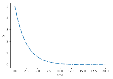
1.2.8 differential equation

from scipy.integrate import odeint

# solve: dy/dt= -0.4y
def dydt(y, t, a):
    return -a * y

a = 0.4
t= np.linspace(0,20)
y0 = 5.0
y = odeint(dydt, y0, t, args=(a,))

fig, ax = plt.subplots()
plt.plot(t, y)
plt.xlabel('time')
plt.ylabel('y')

plt.show()

1.2.9 optimization

\(minx_1x_4(x_1+x_2+x_3)+x_3\) <- objective function

\(s.t.: x_1x_2x_3x_4>=25\) <- inequality constraint

\(x_1^2+x_2^2+x_3^2+x_4^2=40\) <- equality constraint

\(1<=x_1,x_2,x_3,x_4<=5\) <- bounds

\(x_0=(1,5,5,1)\) <- initial guess

from scipy.optimize import minimize
def objective(x):
    x1 = x[0]
    x2 = x[1]
    x3 = x[2]
    x4 = x[3]
    return x1*x4*(x1+x2+x3)+x3

def constraint1(x):
    x1 = x[0]
    x2 = x[1]
    x3 = x[2]
    x4 = x[3]
    return x1*x2*x3*x4-25.0

def constraint2(x):
    sum_sq = 40
    for i in range(4):
        sum_sq = sum_sq - x[i]**2
    return sum_sq

x0 = [1,5,5,1] # initial guess
print (objective(x0))

b = (1.0, 5.0)
bnds = (b, b, b, b)
con1 = {'type': 'ineq', 'fun': constraint1}
con2 = {'type': 'eq', 'fun': constraint2}
cons = [con1, con2]

sol = minimize(objective,
               x0,
               method='SLSQP',
               bounds=bnds,
               constraints=cons)
print (sol)