scikit-笔记20:非监督学习-非线性降维

One weakness of PCA is that it cannot detect non-linear features. A set of algorithms known as Manifold Learning have been developed to address this deficiency. A canonical dataset used in Manifold learning is the S-curve:

from sklearn.datasets import make_s_curve
X, y = make_s_curve(n_samples=1000)
from mpl_toolkits.mplot3d import Axes3D
ax = plt.axes(projection='3d')
ax.scatter3D(X[:, 0], X[:, 1], X[:, 2], c=y)
ax.view_init(10, -60);

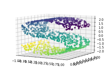
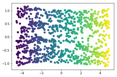
This is a 2-dimensional dataset embedded in three dimensions, but it is embedded in such a way that PCA cannot discover the underlying data orientation:

from sklearn.decomposition import PCA
X_pca = PCA(n_components=2).fit_transform(X)
plt.scatter(X_pca[:, 0], X_pca[:, 1], c=y);

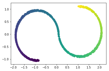
Manifold learning algorithms, however, available in the sklearn.manifold submodule, are able to recover the underlying 2-dimensional manifold:

from sklearn.manifold import Isomap
iso = Isomap(n_neighbors=15, n_components=2)
X_iso = iso.fit_transform(X)
plt.scatter(X_iso[:, 0], X_iso[:, 1], c=y);

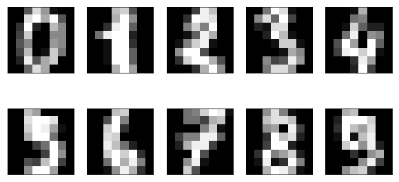
We can apply manifold learning techniques to much higher dimensional datasets, for example the digits data that we saw before:

from sklearn.datasets import load_digits
digits = load_digits()
fig, axes = plt.subplots(2, 5, figsize=(10, 5),
                         subplot_kw={'xticks':(), 'yticks': ()})
for ax, img in zip(axes.ravel(), digits.images):
    ax.imshow(img, interpolation="none", cmap="gray")

8*8 …….. …….. …….. 1*1 …….. -—pca-—> . -—> draw as one point on 2d image to see …….. whether or not we can separate different digits …….. …….. ……..

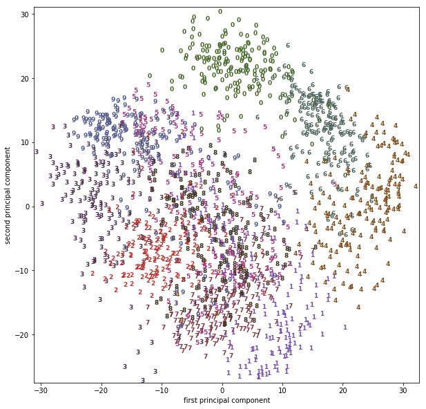
We can visualize the dataset using a linear technique, such as PCA. We saw this already provides some intuition about the data:

# build a PCA model
pca = PCA(n_components=2)
pca.fit(digits.data)
# transform the digits data onto the first two principal components
digits_pca = pca.transform(digits.data)
# setup 10 colors, each color for each digit from 0 ~ 9
colors = ["#476A2A", "#7851B8", "#BD3430", "#4A2D4E", "#875525",
          "#A83683", "#4E655E", "#853541", "#3A3120","#535D8E"]
# setup figsize, x,y limitation
plt.figure(figsize=(10, 10))
plt.xlim(digits_pca[:, 0].min(), digits_pca[:, 0].max() + 1)
plt.ylim(digits_pca[:, 1].min(), digits_pca[:, 1].max() + 1)

# using pca mapping result of each digit image smaple as index;
# using label of each digit image as text you want to draw.
for i in range(len(digits.data)):
    # actually plot the digits as text instead of using scatter
    plt.text(digits_pca[i, 0],                 #<- the x-axis given by model pca
             digits_pca[i, 1],                 #<- the y-axis given by model pca
             str(digits.target[i]),            #<- the digit we want to draw
             color = colors[digits.target[i]], #<- use the true label(0~9) as index of colors array
             fontdict={'weight': 'bold', 'size': 9}
    )
plt.xlabel("first principal component")
plt.ylabel("second principal component");

Using a more powerful, nonlinear techinque can provide much better visualizations, though. Here, we are using the t-SNE manifold learning method:

from sklearn.manifold import TSNE
tsne = TSNE(random_state=42)
# use fit_transform instead of fit, as TSNE has no transform method:
digits_tsne = tsne.fit_transform(digits.data)

import matplotlib.pyplot as plt
import numpy as np
from sklearn.manifold import TSNE
from sklearn.datasets import load_digits
from sklearn.decomposition import PCA
from sklearn.datasets import make_s_curve
from mpl_toolkits.mplot3d import Axes3D
from sklearn.manifold import Isomap

X, y = make_s_curve(n_samples=1000)
X_pca = PCA(n_components=2).fit_transform(X)
iso = Isomap(n_neighbors=15, n_components=2)
X_iso = iso.fit_transform(X)

# build a PCA model
pca = PCA(n_components=2)
pca.fit(digits.data)

# transform the digits data onto the first two principal components
digits_pca = pca.transform(digits.data)
colors = ["#476A2A", "#7851B8", "#BD3430", "#4A2D4E", "#875525",
          "#A83683", "#4E655E", "#853541", "#3A3120","#535D8E"]

# build a TSNE obj
tsne = TSNE(random_state=42)

# use fit_transform instead of fit, as TSNE has no transform method:
# get 2d data points after tsne mapping
digits_tsne = tsne.fit_transform(digits.data)

# set figsize, x,y limitation
plt.figure(figsize=(10, 10))
plt.xlim(digits_tsne[:, 0].min(), digits_tsne[:, 0].max() + 1)
plt.ylim(digits_tsne[:, 1].min(), digits_tsne[:, 1].max() + 1)

# using tsne mapping result of each digit image smaple as index;
# using label of each digit image as text you want to draw.
for i in range(len(digits.data)):
    plt.text(digits_tsne[i, 0],                #<- the x-axis given by model tsne
             digits_tsne[i, 1],                #<- the y-axis given by model tsne
             str(digits.target[i]),            #<- the digit we want to draw
             color = colors[digits.target[i]], #<- use the true label(0~9) as index of colors array
             fontdict={'weight': 'bold', 'size': 9})
plt.show()

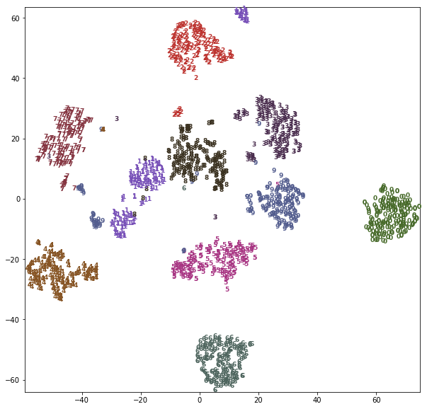
t-SNE has a somewhat longer runtime that other manifold learning algorithms, but the result is quite striking. Keep in mind that this algorithm is purely unsupervised, and does not know about the class labels. Still it is able to separate the classes very well (though the classes four, one and nine have been split into multiple groups).

Here, just use PCA as example to show

model

---

1. build a PCA model,
   1. build obj: pca_obj = PCA()
   2. obj -> model: pca = pca_obj.fit(X_train)

transform

---

1. transform the digits by PCA
   1. pca_data = pca.transform(X_train)

setup plot attr

---

1. setup 10 colors, each color for each digit from 0 ~ 9
   1. colors = ['', '', …, '']
2. setup figsize, x,y limitation
   1. plt.figure(figsize=(10,10))

draw digits

---

1. using pca mapping result of each digit image smaple as index; using label of each digit image as text you want to draw: for i in len(digits.data()): plt.text(….
   1. the x-axis given by model pca
      • pca_data[:,0]
   2. the y-axis given by model pca
      • pca_data[:,1]
   3. the digit we want to draw
      • str = digits.target[i]
   4. use the true label(0~9) as index of colors array
      • c = colors[digits.target[i]]

1. from sklearn.datasets import make_blobs
2. from sklearn.datasets import make_moons
3. from sklearn.datasets import make_circles
4. from sklearn.datasets import make_s_curve *
5. from mpl_toolkits.mplot3d import Axes3D *
6. from sklearn.datasets import make_regression
7. from sklearn.datasets import load_iris
8. from sklearn.datasets import load_digits
9. from sklearn.datasets import load_breast_cancer
10. from sklearn.model_selection import train_test_split
11. from sklearn.model_selection import cross_val_score
12. from sklearn.model_selection import KFold
13. from sklearn.model_selection import StratifiedKFold
14. from sklearn.model_selection import ShuffleSplit
15. from sklearn.model_selection import GridSearchCV
16. from sklearn.model_selection import learning_curve
17. from sklearn.feature_extraction import DictVectorizer
18. from sklearn.feature_extraction.text import CountVectorizer
19. from sklearn.feature_extraction.text import TfidfVectorizer
20. from sklearn.feature_selection import SelectPercentile
21. from sklearn.feature_selection import f_classif
22. from sklearn.feature_selection import f_regression
23. from sklearn.feature_selection import chi2
24. from sklearn.feature_selection import SelectFromModel
25. from sklearn.feature_selection import RFE
26. from sklearn.linear_model import LogisticRegression
27. from sklearn.linear_model import LinearRegression
28. from sklearn.linear_model import Ridge
29. from sklearn.linear_model import Lasso
30. from sklearn.linear_model import ElasticNet
31. from sklearn.neighbors import KNeighborsClassifier
32. from sklearn.neighbors import KNeighborsRegressor
33. from sklearn.preprocessing import StandardScaler
34. from sklearn.metrics import confusion_matrix, accuracy_score
35. from sklearn.metrics import adjusted_rand_score
36. from sklearn.metrics.scorer import SCORERS
37. from sklearn.metrics import r2_score
38. from sklearn.cluster import KMeans
39. from sklearn.cluster import KMeans
40. from sklearn.cluster import MeanShift
41. from sklearn.cluster import DBSCAN # <<< this algorithm has related sources in LIHONGYI's lecture-12
42. from sklearn.cluster import AffinityPropagation
43. from sklearn.cluster import SpectralClustering
44. from sklearn.cluster import Ward
45. from sklearn.cluster import DBSCAN
46. from sklearn.cluster import AgglomerativeClustering
47. from scipy.cluster.hierarchy import linkage
48. from scipy.cluster.hierarchy import dendrogram
49. from sklearn.metrics import confusion_matrix
50. from sklearn.metrics import accuracy_score
51. from sklearn.metrics import adjusted_rand_score
52. from sklearn.metrics import classification_report
53. from sklearn.preprocessing import Imputer
54. from sklearn.dummy import DummyClassifier
55. from sklearn.pipeline import make_pipeline
56. from sklearn.svm import LinearSVC
57. from sklearn.svm import SVC
58. from sklearn.tree import DecisionTreeRegressor
59. from sklearn.ensemble import RandomForestClassifier
60. from sklearn.ensemble import GradientBoostingRegressor
61. from sklearn.decomposition import PCA *
62. from sklearn.manifold import TSNE *
63. from sklearn.manifold import Isomap *

from mpl_toolkits.mplot3d import Axes3D *