lec 03 Perceptron Algorithm and Hard-SVM
Table of Contents
- Gradient descent,
- stochastic gradient descent,
- and the perceptron learning algorithm.
- Feature space versus weight space.
- The maximum margin classifier,
- aka hard-margin support vector machine (SVM).
Perceptron Algorithm (cont'd)
Recall:
- linear predictor fn f(x) = w . x   (for simplicity, no alpha)
- decision boundary {x : f(x) = 0}   (a hyperplane through the origin)

- samples X_1, X_2, ..., X_n (vectors); classifications y_1, ..., y_n = +- 1
- goal:  find weights w such that y_i X_i . w >= 0
- goal, rewritten:  find w that minimizes R(w) = sum -y_i X_i . w     [risk fn]
                                         i in V
                    where V is the set of indicies i for which y_i X_i . w < 0.
[Our original problem was to find a separating hyperplane in one space, which I'll call x-space. But we've transformed this into a problem of finding an optimal point in a different space, which I'll call w-space. It's important to understand transformations like this, where a structure in one space becomes a point in another space. In this particular problem, there is a duality between hyperplanes and points.]
Duality between x-space and w-space:
        x-space (primal)                w-space (dual)
|---------------------------------------------------------------|
|  hyperplane:  {z : w . z = 0} |  point:       w               |
|---------------------------------------------------------------|
|  point:       x               |  hyperplane:  {z : x . z = 0} |
|---------------------------------------------------------------|
If a point x lies on a hyperplane H, then its dual hyperplane x^* contains the dual point H^*. 我的面是你的点,你的点是我的面。通过这个规律,我们要求自己这边的面,就先约束自己的点,然后映射到你的面,在通过约束你的面得到你的约束点,再把你的约束点映射回我的约束面。
        x-space        .         w-space
                       .
      **        vector ⊥ plane         /------------
      ** --------------.------------>  /           /
       |               .              /           /
       |               .             /           /
     \ | /             .            ------+-----/
      \|/              .                  |
       X               .                  |
      /|\              .                  |
     / | \             .              vector ∈ plane
       |               .                  |
       v               .                  |
    /---------/        .                  |
   /         /         .                  |
  /         /          .                  v
 /         /  <--------.----------------- **
/----------      plane ⊥ vector           **
                       .
Duality 到底是什么?说白了就是 坐标系 变换:
- 原来坐标系(x-space)的坐标轴是:feature_1,feature_2,feature_3…
- 新的坐标系(w-space)的坐标轴是:w_1, w_2, w_3…
- 而且根据 constraint,w.x=0
同一个函数 yi(w.xi)>=0 用不同的坐标系就会绘出不一样的图形。巧的是如果使用 x-space 坐标系,其中的点在 w-space 恰好是面;其中的面在 w-space 恰好是点。
现在已知 x-space 的点,求 x-space 的面 我就把问题转化为: 现在已知 w-space 的面,求 w-space 的点 而且,因为 w.x=0 的限制条件,所以 x-space 的点(向量)与 w-space 的面垂直;反之亦然
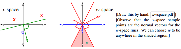
Observe that the x-space sample points are the normal vectors for the w-space lines. We can choose w to be anywhere in the shaded region
原问题空间中求 hyperplane{x:x.w=0}范围的问题,通过 dual 转换为上图中求 w 向量范围的问题(灰色区域是 w 向量的取值范围)。
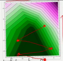
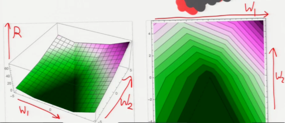 这个 plot 是关于 R(w) 在 w-space 的图像。可以看到,深绿色区域是 R(w) = 0 的点。这里假设 w 是二维向量。
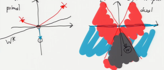
If we want to enforce inequality x . w >= 0, that means
  - x should be on the correct side of {z : z . w = 0} in primal x-space
  - w   "    "  "   "     "     "   "  {z : x . z = 0} in dual w-space

                 ^                    \    ^    /
    primal       |        X            \   |   /   dual
                 |                      \  |  /
            X    |      ----             \ | /            [Observe that the
                 |  ----                  \|/              primal points are
       <---------+--------->     <=========+=========>     the normal vectors
           ----  |                        /|\              for the dual lines.]
       ----      |                       / | \
                 0                      /  |  \
                 |                     /   | w \
                 v                    /    v    \
[For a sample x in class O, w and x must be on the same side of the dual hyperplane x^*. For a sample x not in class O (X), w and x must be on opposite sides of the dual hyperplane x^*.]
[Show plots of R. Note how R's creases match the dual chart.]
[In this example, we can choose w to be any point in the bottom pizza slice; all those points satisfy the inequalities.]
[We have an optimization problem; we need an optimization algorithm to solve it.]
An optimization algorithm: gradient descent on R.
问题演变为如何最小化 R(w), 可以用求导法来求极值,也可以用这里的梯度下降法来求极值。
How to minimize a function: -grad(fn)
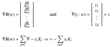
Given a starting point w, find gradient of R with respect to w; this is the direction of steepest ascent. Take a step in the opposite direction. Recall [from your vector calculus class]
            -         -                           -     -
            | dR/dw_1 |                           | z_1 |
            |         |                           |     |
grad R(w) = | dR/dw_2 |     and    grad (z . w) = | z_2 | = z.
            |    .    |                           |  .  |
            |    .    |                           |  .  |
            | dR/dw_d |                           | z_d |
            -         -                           -     -

grad R(w) = sum  grad -y_i X_i . w = - sum  y_i X_i
           i in V                     i in V
注意:反梯度法的 loss-fn 是要计算所有样本的误差之和
这里梯度 grad R(w) 得到的是一个 R(w) 以最快速度变大的方向, 所以如果我希望 R(w) 以最快速度变小,那么就应该朝梯度的反方向移动点 w(或叫向量 w), 梯度的反向就是负梯度:- Grad[R(w)], 这就是梯度下降法或叫 负梯度法 。
At any point w, we walk downhill in direction of steepest descent, - grad R(w).
Algo: gradient descent
w = arbitrary nonzero starting point (good choice is any y_i X_i)
while R(w) > 0
  V <- set of indicies i for which y_i X_i . w < 0   // 这里从公式 - y_i X_i . w > 0 转化得到
  w <- w + epsilon sum  y_i X_i                      // 这里更普适的写法是: w = w + 负梯度增量
                  i in V
return w
上述算法中,每一次更新向量 w,都会让 w 朝 R(w)=0 的区域前进一点,所以要注意调整 learning rate。下图中每一次转折,都代表一次 w 的更新, 可以看到这个点是从 R(w)>0 浅绿色 ====> R(w)=0 深绿色移动的。
Learning rate, step size
epsilon is the step_size aka learning_rate, chosen empirically. [Best choice depends on input problem!]
[Show plot of R again. Show typical steps.]
Running time of Gradient descent algo
Problem: Slow! Each step takes O(nd) time. 因为 所有 sample 都要检测 y_i X_i . w <? 0 ,而 w 向量又是 d 维的。所以单次循环的时间复杂度是:O(nd)
- n 表示有 n 个样本;
- d 表示有 d 个 feature; 一个 feature 表示一维度。
注意:反梯度法的 loss-fn 是要计算所有样本的误差之和
Improvement: Perceptron algo (SGD)
Optimization algorithm 2: Stochastic Gradient Descent
Idea: each step, pick one misclassified X_i; do gradient descent on loss fn L(X_i . w, y_i).
Called the perceptron_algorithm. Each step takes O(d) time. [Not counting the time to search for a misclassified X_i.]
algo: perceptron
注意:反梯度法的 loss-fn 是要计算所有样本的误差之和 GD 反梯度法 单步循环 是 all-sample one-modification2w SGD 随机反梯度法 单步循环 是 one-sample one-modification2w
因为在执行每次更新时,我们需要在整个数据集上计算所有的梯度,所以批梯度下降法的速度会很慢,同时,批梯度下降法无法处理超出内存容量限制的数据集。批梯度下降法同样也不能在线更新模型,即在运行的过程中,不能增加新的样本。
while some y_i X_i . w < 0
  w <- w + epsilon y_i X_i
return w
w = arbitrary nonzero starting point (good choice is any y_i X_i)
while R(w) > 0
  V <- set of indicies i for which y_i X_i . w < 0   // 这里从公式 - y_i X_i . w > 0 转化得到
  w <- w + epsilon sum  y_i X_i                      // 这里更普适的写法是: w = w + 负梯度增量
                  i in V
return w
when SGD work well: loss-fn must be convex
SGD 虽然更快更灵活能在线添加样本,但是没有 GD 的适用范围广。GD 能处理的问题,SGD 未必能处理。
In general, you CAN NOT assume that if you optimize a sum of fn that you can optimize each fn separately in turn and find a minimum of the sum.
The reason SGD works in this particular case is because the loss fn has a very nice property called convexity. The sum of a bunch of convex fn is convex and that's what makes SGD work
这里的意思是说,如果 loss-fn 是凸函数,那么就是可以使用 SGD,如果不是,就不能用 SGD。
[By the way, stochastic gradient descent does not work for every problem that gradient descent works for. The perceptron risk function happens to have special properties that allow stochastic gradient descent to always succeed.]
Advantage of SGD: online algo
[One interesting aspect of the perceptron algorithm is that it's an "online algorithm", which means that if new data points come in while the algorithm is already running, you can just throw them into the mix and keep looping.]
Perceptron Convergence Theorem
Perceptron Convergence Theorem: If data is linearly separable, perceptron algorithm will find a linear classifier that classifies all data correctly in at most O(R^2 / gamma^2) iterations, where R = max |X_i| is "radius of data" and gamma is the "maximum margin". [I'll define "maximum margin" shortly.]
We're not going to prove this, because it's obsolete.]
Although the step size/learning rate doesn't appear in that big-O expression, it does have an effect on the running time, but the effect is hard to characterize.
Problem of step size(learning rate)
SGD is also get slower
The algorithm gets slower if:
- epsilon is too small because it has to take lots of steps to get down the hill
- epsilon is too big for a different reason: it jumps right over the region with zero risk and oscillates back and forth for a long time.
hard to choose a good step size
Although stochastic gradient descent is faster for this problem than gradient descent, the perceptron algorithm is still slow.
There's no reliable way to choose a good step size epsilon.
Fortunately, optimization algorithms have improved a lot since 1957. You can get rid of the step size by using any decent modern "line search" algorithm. Better yet, you can find a better decision boundary much more quickly by quadratic programming, which is what we'll talk about next.
升维法:What if separating hyperplane doesn't pass through origin?
升维法,也是 TsingHua-Datamining chap4 ppt page6 中为什么会有 x_0 w_0 的原因
如果 [超平面] 不过原点,那么就通过 [升维] 把问题转化为 [经过原点] 的问题
if separating hyperplane doesn't pass through orighin, what we do is there are many tricks in optimization where you add a dimension or two to problem, so your space gets one or two dimensions bigger in order to accommodate some trick.
Add a fictitious dimension.
  Hyperplane:  w . x + alpha = 0

                        -     -
                        | x_1 |
    [ w_1 w_2 alpha ] . | x_2 | = 0
                        |  1  |
                        -     -
           |               |
           |               |
           v               v
        new 'w'         new 'x'
              \            /
               v          v
              +--------------+
              |  w' . x' = 0 |
              +--------------+

                        d + 1
Now we have samples in R     , all lying on plane x      = 1.
                                                   d + 1
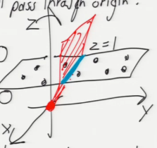
样本原本有 2 个特征:x,y。所有样本点都分在一个平面上。通过增一个维度变成三维空间,这样所有的点仍然都处在原来的那个平面上,只不过这个平面在新空间表示为: X_d+1 = 1 我要做的是在这个空间中使用 SGD or GD 算法得到 w', 然后去掉最后一位得到 w。这个 w,相当于原来的 w' 平面与 X_d+1 = 1 平面的交线.
Run perceptron algorithm in (d + 1)-dimensional space.
[The perceptron algorithm was invented in 1957 by Frank Rosenblatt at the Cornell Aeronautical Laboratory. It was originally designed not to be a program, but to be implemented in hardware for image recognition on a 20 x 20 pixel image. Rosenblatt built a Mark I Perceptron Machine that ran the algorithm, complete with electric motors to do weight updates.]
[Show Mark I photo. This is what it took to process a 20 x 20 image in 1957.]
[Then he had a press conference where he predicted that perceptrons would be "the embryo of an electronic computer that [the Navy] expects will be able to walk, talk, see, write, reproduce itself and be conscious of its existence." We're still waiting on that.]
梯度下降法的变形形式
这里请先参考 Tsinghua-Datamining 课程课件:chap4 Neural Networks-ppt@10
梯度下降法有 3 中变形形式,它们之间的区别为我们在计算目标函数的梯度时使用到多少数据。根据数据量的不同,我们在参数更新的精度和更新过程中所需要的时间两个方面做出权衡。
2.1 批梯度下降法
Vanilla 梯度下降法,又称为批梯度下降法(batch gradient descent),在整个训练数据集上计算损失函数关于参数θ的梯度:
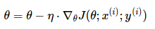
θ=θ − η ⋅ ∇θJ(θ)
因为在执行每次更新时,我们需要在整个数据集上计算所有的梯度,所以批梯度下降法的速度会很慢,同时,批梯度下降法无法处理超出内存容量限制的数据集。批梯度下降法同样也不能在线更新模型,即在运行的过程中,不能增加新的样本。
批梯度下降法的代码如下所示:
for i in range(nb_epochs):
    params_grad = evaluate_gradient(loss_function, data, params)
    params = params - learning_rate * params_grad
然后,我们利用梯度的方向和学习率更新参数,学习率决定我们将以多大的步长更新参数。对于凸误差函数,批梯度下降法能够保证收敛到全局最小值,对于非凸函数,则收敛到一个局部最小值。
2.2 随机梯度下降法
相反,随机梯度下降法(stochastic gradient descent, SGD)根据每一条训练样本 x(i)和标签 y(i)更新参数:
对于大数据集,因为批梯度下降法在每一个参数更新之前,会对相似的样本计算梯度,所以在计算过程中会有冗余。而 SGD 在每一次更新中只执行一次,从而消除了冗余。因而,通常 SGD 的运行速度更快,同时,可以用于在线学习。SGD 以高方差频繁地更新,导致目标函数出现如图 1 所示的剧烈波动。
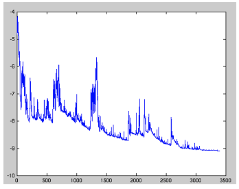 图 1:SGD 波动(来源:Wikipedia)
与批梯度下降法的收敛会使得损失函数陷入局部最小相比,由于 SGD 的波动性,一方面,波动性使得 SGD 可以跳到新的和潜在更好的局部最优。另一方面,这使得最终收敛到特定最小值的过程变得复杂,因为 SGD 会一直持续波动。然而,已经证明当我们缓慢减小学习率,SGD 与批梯度下降法具有相同的收敛行为,对于非凸优化和凸优化,可以分别收敛到局部最小值和全局最小值。与批梯度下降的代码相比,SGD 的代码片段仅仅是在对训练样本的遍历和利用每一条样本计算梯度的过程中增加一层循环。注意,如 6.1 节中的解释,在每一次循环中,我们打乱训练样本。
for i in range(nb_epochs):
    np.random.shuffle(data)
    for example in data:
        params_grad = evaluate_gradient(loss_function, example, params)
        params = params - learning_rate * params_grad
2.3 小批量梯度下降法
小批量梯度下降法最终结合了上述两种方法的优点,在每次更新时使用 n 个小批量训练样本:
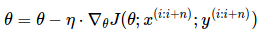
这种方法,a)减少参数更新的方差,这样可以得到更加稳定的收敛结果;b)可以利用最新的深度学习库中高度优化的矩阵优化方法,高效地求解每个小批量数据的梯度。通常,小批量数据的大小在 50 到 256 之间,也可以根据不同的应用有所变化。当训练神经网络模型时,小批量梯度下降法是典型的选择算法,当使用小批量梯度下降法时,也将其称为 SGD。注意:在下文的改进的 SGD 中,为了简单,我们省略了参数 x(i:i+n);y(i:i+n)。
在代码中,不是在所有样本上做迭代,我们现在只是在大小为 50 的小批量数据上做迭代:
for i in range(nb_epochs):
    np.random.shuffle(data)
    for batch in get_batches(data, batch_size=50):
        params_grad = evaluate_gradient(loss_function, batch, params)
        params = params - learning_rate * params_grad
3 挑战
虽然 Vanilla 小批量梯度下降法并不能保证较好的收敛性,但是需要强调的是,这也给我们留下了如下的一些挑战:
- 选择一个合适的学习率可能是困难的。学习率太小会导致收敛的速度很慢,学习率太大会妨碍收敛,导致损失函数在最小值附近波动甚至偏离最小值。
- 学习率调整[17]试图在训练的过程中通过例如退火的方法调整学习率,即根据预定义的策略或者当相邻两代之间的下降值小于某个阈值时减小学习率。然而,策略和阈值需要预先设定好,因此无法适应数据集的特点[4]。
- 此外,对所有的参数更新使用同样的学习率。如果数据是稀疏的,同时,特征的频率差异很大时,我们也许不想以同样的学习率更新所有的参数,对于出现次数较少的特征,我们对其执行更大的学习率。
- 高度非凸误差函数普遍出现在神经网络中,在优化这类函数时,另一个关键的挑战是使函数避免陷入无数次优的局部最小值。Dauphin 等人[5]指出出现这种困难实际上并不是来自局部最小值,而是来自鞍点,即那些在一个维度上是递增的,而在另一个维度上是递减的。这些鞍点通常被具有相同误差的点包围,因为在任意维度上的梯度都近似为 0,所以 SGD 很难从这些鞍点中逃开。
梯度下降优化算法
这里请先参考 Tsinghua-Datamining 课程课件:chap4 Neural Networks-ppt@28
下面,我们将列举一些算法,这些算法被深度学习社区广泛用来处理前面提到的挑战。我们不会讨论在实际中不适合在高维数据集中计算的算法,例如诸如牛顿法的二阶方法。
4.1 动量法
SGD 很难通过陡谷,即在一个维度上的表面弯曲程度远大于其他维度的区域[19],这种情况通常出现在局部最优点附近。在这种情况下,SGD 摇摆地通过陡谷的斜坡,同时,沿着底部到局部最优点的路径上只是缓慢地前进,这个过程如图 2a 所示。
这里写图片描述
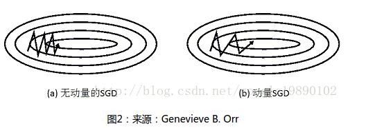 图 2:来源:Genevieve B. Orr
如图 2b 所示,动量法[16]是一种帮助 SGD 在相关方向上加速并抑制摇摆的一种方法。动量法将历史步长的更新向量的一个分量γ增加到当前的更新向量中(部分实现中交换了公式中的符号)
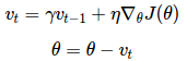
vt=γvt−1+η∇θJ(θ)

θ=θ−vt
动量项γ通常设置为 0.9 或者类似的值。
从本质上说,动量法,就像我们从山上推下一个球,球在滚下来的过程中累积动量,变得越来越快(直到达到终极速度,如果有空气阻力的存在,则γ<1)。同样的事情也发生在参数的更新过程中:对于在梯度点处具有相同的方向的维度,其动量项增大,对于在梯度点处改变方向的维度,其动量项减小。因此,我们可以得到更快的收敛速度,同时可以减少摇摆。
4.2 Nesterov 加速梯度下降法
然而,球从山上滚下的时候,盲目地沿着斜率方向,往往并不能令人满意。我们希望有一个智能的球,这个球能够知道它将要去哪,以至于在重新遇到斜率上升时能够知道减速。
Nesterov 加速梯度下降法(Nesterov accelerated gradient,NAG)[13]是一种能够给动量项这样的预知能力的方法。我们知道,我们利用动量项γvt−1 来更新参数θ。通过计算θ−γvt−1 能够告诉我们参数未来位置的一个近似值(梯度并不是完全更新),这也就是告诉我们参数大致将变为多少。通过计算关于参数未来的近似位置的梯度,而不是关于当前的参数θ的梯度,我们可以高效的求解 :
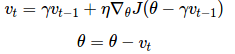
vt=γvt−1+η∇θJ(θ−γvt−1)

θ=θ−vt
同时,我们设置动量项γ大约为 0.9。动量法首先计算当前的梯度值(图 3 中的小的蓝色向量),然后在更新的累积梯度(大的蓝色向量)方向上前进一大步,Nesterov 加速梯度下降法 NAG 首先在先前累积梯度(棕色的向量)方向上前进一大步,计算梯度值,然后做一个修正(绿色的向量)。这个具有预见性的更新防止我们前进得太快,同时增强了算法的响应能力,这一点在很多的任务中对于 RNN 的性能提升有着重要的意义[2]。
这里写图片描述
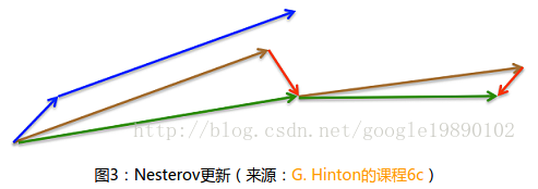 图 3:Nesterov 更新(来源:G. Hinton 的课程 6c)
对于 NAG 的直观理解的另一种解释可以参见 http://cs231n.github.io/neural-networks-3/,同时 Ilya Sutskever 在其博士论文 [18]中给出更详细的综述。
既然我们能够使得我们的更新适应误差函数的斜率以相应地加速 SGD,我们同样也想要使得我们的更新能够适应每一个单独参数,以根据每个参数的重要性决定大的或者小的更新。
4.3 Adagrad
Adagrad[7]是这样的一种基于梯度的优化算法:让学习率适应参数,对于出现次数较少的特征,我们对其采用更大的学习率,对于出现次数较多的特征,我们对其采用较小的学习率。因此,Adagrad 非常适合处理稀疏数据。Dean 等人[6]发现 Adagrad 能够极大提高了 SGD 的鲁棒性并将其应用于 Google 的大规模神经网络的训练,其中包含了 YouTube 视频中的猫的识别。此外,Pennington 等人[15]利用 Adagrad 训练 Glove 词向量,因为低频词比高频词需要更大的步长。
前面,我们每次更新所有的参数θ时,每一个参数θi 都使用的是相同的学习率η。由于 Adagrad 在 t 时刻对每一个参数θi 使用了不同的学习率,我们首先介绍 Adagrad 对每一个参数的更新,然后我们对其向量化。为了简洁,令 gt,i 为在 t 时刻目标函数关于参数θi 的梯度:
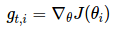
gt,i=∇θJ(θi)
在 t 时刻,对每个参数θi 的更新过程变为:
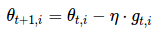
θt+1,i=θt,i−η⋅gt,i
对于上述的更新规则,在 t 时刻,基于对θi 计算过的历史梯度,Adagrad 修正了对每一个参数θi 的学习率:
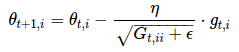
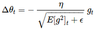
θt+1,i=θt,i−ηGt,ii+ϵ−−−−−−−√⋅gt,i
其中,Gt∈Rd×d 是一个对角矩阵,对角线上的元素 i,i 是直到 t 时刻为止,所有关于θi 的梯度的平方和(Duchi 等人[7]将该矩阵作为包含所有先前梯度的外积的完整矩阵的替代,因为即使是对于中等数量的参数 d,矩阵的均方根的计算都是不切实际的。),ϵ是平滑项,用于防止除数为 0(通常大约设置为 1e−8)。比较有意思的是,如果没有平方根的操作,算法的效果会变得很差。
由于 Gt 的对角线上包含了关于所有参数θ的历史梯度的平方和,现在,我们可以通过 Gt 和 gt 之间的元素向量乘法⊙向量化上述的操作:
θt+1=θt−ηGt+ϵ−−−−−√⊙gt
Adagrad 算法的一个主要优点是无需手动调整学习率。在大多数的应用场景中,通常采用常数 0.01。
Adagrad 的一个主要缺点是它在分母中累加梯度的平方:由于没增加一个正项,在整个训练过程中,累加的和会持续增长。这会导致学习率变小以至于最终变得无限小,在学习率无限小时,Adagrad 算法将无法取得额外的信息。接下来的算法旨在解决这个不足。
4.4 Adadelta
Adadelta[21]是 Adagrad 的一种扩展算法,以处理 Adagrad 学习速率单调递减的问题。不是计算所有的梯度平方,Adadelta 将计算计算历史梯度的窗口大小限制为一个固定值 w。
在 Adadelta 中,无需存储先前的 w 个平方梯度,而是将梯度的平方递归地表示成所有历史梯度平方的均值。在 t 时刻的均值 E[g2]t 只取决于先前的均值和当前的梯度(分量γ类似于动量项):
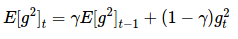
E[g2]t=γE[g2]t−1+(1−γ)g2t
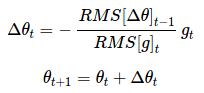
我们将γ设置成与动量项相似的值,即 0.9 左右。为了简单起见,我们利用参数更新向量Δθt 重新表示 SGD 的更新过程:
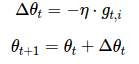
    Δθt=−η⋅gt,i

    θt+1=θt+Δθt
我们先前得到的 Adagrad 参数更新向量变为:
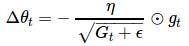
Δθt=−ηGt+ϵ−−−−−√⊙gt
现在,我们简单将对角矩阵 Gt 替换成历史梯度的均值 E[g2]t:
Δθt=−ηE[g2]t+ϵ−−−−−−−−√gt
由于分母仅仅是梯度的均方根(root mean squared,RMS)误差,我们可以简写为:
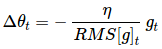
Δθt=−ηRMS[g]tgt
作者指出上述更新公式中的每个部分(与 SGD,动量法或者 Adagrad)并不一致,即更新规则中必须与参数具有相同的假设单位。为了实现这个要求,作者首次定义了另一个指数衰减均值,这次不是梯度平方,而是参数的平方的更新:
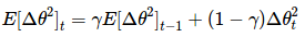
E[Δθ2]t=γE[Δθ2]t−1+(1−γ)Δθ2t
因此,参数更新的均方根误差为:
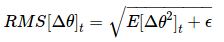
RMS[Δθ]t=E[Δθ2]t+ϵ−−−−−−−−−√
由于 RMS[Δθ]t 是未知的,我们利用参数的均方根误差来近似更新。利用 RMS[Δθ]t−1 替换先前的更新规则中的学习率η,最终得到 Adadelta 的更新规则:
    Δθt=−RMS[Δθ]t−1RMS[g]tgt

    θt+1=θt+Δθt
使用 Adadelta 算法,我们甚至都无需设置默认的学习率,因为更新规则中已经移除了学习率。
4.5 RMSprop
RMSprop 是一个未被发表的自适应学习率的算法,该算法由 Geoff Hinton 在其 Coursera 课堂的课程 6e 中提出。
RMSprop 和 Adadelta 在相同的时间里被独立的提出,都起源于对 Adagrad 的极速递减的学习率问题的求解。实际上,RMSprop 是先前我们得到的 Adadelta 的第一个更新向量的特例:
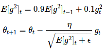
E[g2]t=0.9E[g2]t−1+0.1g2t

θt+1=θt−ηE[g2]t+ϵ−−−−−−−−√gt
同样,RMSprop 将学习率分解成一个平方梯度的指数衰减的平均。Hinton 建议将γ设置为 0.9,对于学习率η,一个好的固定值为 0.001。
4.6 Adam
自适应矩估计(Adaptive Moment Estimation,Adam)[9]是另一种自适应学习率的算法,Adam 对每一个参数都计算自适应的学习率。除了像 Adadelta 和 RMSprop 一样存储一个指数衰减的历史平方梯度的平均 vt,Adam 同时还保存一个历史梯度的指数衰减均值 mt,类似于动量:
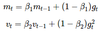
mt=β1mt−1+(1−β1)gt

vt=β2vt−1+(1−β2)g2t
mt 和 vt 分别是对梯度的一阶矩(均值)和二阶矩(非确定的方差)的估计,正如该算法的名称。当 mt 和 vt 初始化为 0 向量时,Adam 的作者发现它们都偏向于 0,尤其是在初始化的步骤和当衰减率很小的时候(例如β1 和β2 趋向于 1)。
通过计算偏差校正的一阶矩和二阶矩估计来抵消偏差:
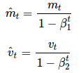
m^t=mt1−βt1

v^t=vt1−βt2
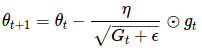
正如我们在 Adadelta 和 RMSprop 中看到的那样,他们利用上述的公式更新参数,由此生成了 Adam 的更新规则:
θt+1=θt−ηv^t−−√+ϵm^t
作者建议β1 取默认值为 0.9,β2 为 0.999,ϵ为 10−8。他们从经验上表明 Adam 在实际中表现很好,同时,与其他的自适应学习算法相比,其更有优势。
4.7 算法可视化
下面两张图给出了上述优化算法的优化行为的直观理解。(还可以看看这里关于 Karpathy 对相同的图片的描述以及另一个简明关于算法讨论的概述)。
在图 4a 中,我们看到不同算法在损失曲面的等高线上走的不同路线。所有的算法都是从同一个点出发并选择不同路径到达最优点。注意:Adagrad,Adadelta 和 RMSprop 能够立即转移到正确的移动方向上并以类似的速度收敛,而动量法和 NAG 会导致偏离,想像一下球从山上滚下的画面。然而,NAG 能够在偏离之后快速修正其路线,因为 NAG 通过对最优点的预见增强其响应能力。
图 4b 中展示了不同算法在鞍点处的行为,鞍点即为一个点在一个维度上的斜率为正,而在其他维度上的斜率为负,正如我们前面提及的,鞍点对 SGD 的训练造成很大困难。这里注意,SGD,动量法和 NAG 在鞍点处很难打破对称性,尽管后面两个算法最终设法逃离了鞍点。而 Adagrad,RMSprop 和 Adadelta 能够快速想着梯度为负的方向移动,其中 Adadelta 走在最前面。
SGD without momentum (a)损失去面的等高线上 SGD 优化
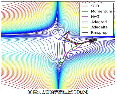
SGD with momentum (b)在鞍点处的 SGD 优化
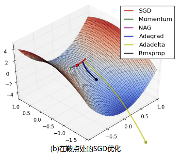 图 4:来源和全部动画:Alec Radford
正如我们所看到的,自适应学习速率的方法,即 Adagrad、Adadelta、RMSprop 和 Adam,最适合这些场景下最合适,并在这些场景下得到最好的收敛性。
4.8 选择使用哪种优化算法?
那么,我们应该选择使用哪种优化算法呢?如果输入数据是稀疏的,选择任一自适应学习率算法可能会得到最好的结果。选用这类算法的另一个好处是无需调整学习率,选用默认值就可能达到最好的结果。
总的来说,RMSprop 是 Adagrad 的扩展形式,用于处理在 Adagrad 中急速递减的学习率。 RMSprop 与 Adadelta 相同,所不同的是 Adadelta 在更新规则中使用参数的均方根进行更新。最后,Adam 是将偏差校正和动量加入到 RMSprop 中。在这样的情况下,RMSprop、 Adadelta 和 Adam 是很相似的算法并且在相似的环境中性能都不错。Kingma 等人[9]指出在优化后期由于梯度变得越来越稀疏,偏差校正能够帮助 Adam 微弱地胜过 RMSprop。综合看来,Adam 可能是最佳的选择。
有趣的是,最近许多论文中采用不带动量的 SGD 和一种简单的学习率的退火策略。已表明,通常 SGD 能够找到最小值点,但是比其他优化的 SGD 花费更多的时间,与其他算法相比,SGD 更加依赖鲁棒的初始化和退火策略,同时,SGD 可能会陷入鞍点,而不是局部极小值点。因此,如果你关心的是快速收敛和训练一个深层的或者复杂的神经网络,你应该选择一个自适应学习率的方法。
MAXIMUM MARGIN CLASSIFIERS
========================
The margin of a linear classifier is the distance from the decision boundary
to the nearest sample point. What if we make the margin as big as possible?
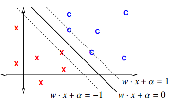
new constraint
Margin 是分界面 hyperplane 到最近点的垂直距离,所以有两个 margin,一边一个。由上图 -1 <= Margin <= 1 可以用同样的方法推导出新的 constraint 公式:
[Notice that the right-hand side is a 1, rather than a 0 as it was for the perceptron risk function. It's not obvious, but this a much better way to formulate the problem, partly because it makes it impossible for the weight vector w to get set to zero.]
from constraint to margin
If w is a unit vector, |w| = 1, the constraints imply the margin is at least 1;
  [because w . X_i + alpha is the signed distance] signed distance 的意思是说

                                                                    1
BUT we allow w to have arbitrary length, so the margin is at least ---.
                                                                   |w|
                                                     不等式两边同除以|w|得到

                            2
There is a _slab_ of width --- containing no samples
                           |w|
[with the hyperplane running along its middle].
from constraint to new optimization problem
To maximize the margin, minimize |w|. Optimization problem:
----------------------------------------------------------------
| Find w and alpha that minimize |w|^2                         |
| subject to y_i (X_i . w + alpha) >= 1    for all i in [1, n] |
----------------------------------------------------------------
Called a quadratic_program in d + 1 dimensions and n constraints. It has one unique solution!
Why use |w|^2 instead of |w|? [The reason we use |w|^2 as an objective function, instead of |w|, is that the length function |w| is not smooth at zero, whereas |w|^2 is smooth everywhere.]
The solution gives us a maximum_margin_classifier, aka a hard_margin support_vector_machine (SVM).
[Technically, this isn't really a support vector machine yet; it doesn't fully deserve that name until we add features and kernelization, which we'll do in later lectures.]
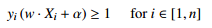
[Show 3D example in (w, alpha) weight space + 2D cross-section w1 = 1/17. Show optimal point on both graphs.]
This is an example of what the linear constraints look like in the 3D weight space (w1,w2,α) for an SVM with three training points.
The SVM is looking for the point nearest the origin that lies above the blue plane (representing an inclass training point) but below the red and pink planes (representing out-of-class training points).
In this example, that optimal point lies where the three planes intersect. At right we see a 2D cross-section w1 = 1/17 of the 3D space, because the optimal solution lies in this cross-section.
The constraints say that the solution must lie in the leftmost pizza slice, while being as close to the origin as possible, so the optimal solution is where the three lines meet.
用之前的图(如下)对比理解,上图仅仅展示了 w-space 空间的样子; 而下图左边是 x-space, 右边是 w-space。