lec 05 Hierarchical of ML and Optimization Problem
Table of Contents
lec 05 Hierarchical of ML and Optimization Problem
ML ABSTRACTIONS [some meta comments on machine learning]
=============
[When you write a large computer program, you break it down into subroutines
and modules. Many of you know from experience that you need to have the
discipline to impose strong abstraction barriers between different modules, or
your program will become so complex you can no longer manage nor maintain it.]
[When you learn a new subject, it helps to have mental abstraction barriers, too, so you know when you can replace one approach with a different approach. I want to give you four levels of abstraction that can help you think about machine learning. It's important to make mental distinctions between these four things, and the code you write should have modules that reflect these distinctions as well.]
-----------------------------------------------------------------------------
| APPLICATION/DATA                                                          |
|                                                                           |
| data labeled (classified) or not?                                         |
| yes: labels categorical (classification) or quantitative (regression)?    |
| no:  _similarity_ (clustering) or positioning (dimensionality reduction)? |
|---------------------------------------------------------------------------|
| MODEL                           [what kinds of hypotheses are permitted?] |
|                                                                           |
| e.g.:                                                                     |
| - predictor fns:  linear, polynomial, logistic, neural net, ...           |
| - nearest neighbors, decision trees(have no predictor fn)                 |
| - features                                                                |
| - low vs. high capacity (affects overfitting, underfitting, inference)    |
|---------------------------------------------------------------------------|
| OPTIMIZATION PROBLEM                                                      | a molde can be optimized by many OPTIMIZATION PROBLEM
|                                                                           | a OPTIMIZATION PROBLEM always can be expressed with
| - variables, objective fn, constraints                                    | 3 key-terms: var, obj, contr
| e.g., unconstrained, convex program, least squares, PCA                   |
|---------------------------------------------------------------------------|
| OPTIMIZATION ALGORITHM                                                    | an OPTIMIZATION PROBLEM can be solved by many
|                                                                           | OPTIMIZATION ALGORITHMS
| e.g., gradient descent, simplex, SVD                                      | (简单理解为求 极大/小值)
-----------------------------------------------------------------------------
[In this course, we focus primarily on the middle two levels. As a data scientist, you might be given an application, and your challenge is to turn it into an optimization problem that we know how to solve. We'll talk a bit about optimization algorithms, but usually you'll use an optimization code that's faster and more robust than what you would write.
[The second level, the model, has a huge effect on the success of your learning algorithm. Sometimes you can get a big improvement by tailoring the model or its features to fit the structure of your specific data. The model also has a big effect on whether you overfit or underfit. And if you want a model that you can interpret so you can do inference, the model has to be regular, not too complex. Lastly, you have to pick a model that leads to an optimization problem that can be solved. Some optimization problems are just too hard.]
[It's important to understand that when you change something in one level of this diagram, you probably have to change all the levels underneath it. If you switch from a linear classifier to a neural net, your optimization problem changes, and your optimization algorithm probably changes too.]
[Not all machine learning methods fit this four-level decomposition. Nevertheless, for everything you learn in this class, think about where it fits in this hierarchy. If you don't distinguish which math is part of the model and which math is part of the optimization algorithm, this course will be very confusing for you.]
OPTIMIZATION PROBLEMS
===================
[I want to familiarize you with some types of optimization problems that can be
solved reliably and efficiently, and the names of some of the optimization
algorithms used to solve them. An important skill for you to develop is to be
able to go from an application to a well-defined optimization problem.]
Unconstrained Optimization
根据,AMATH301 课程提示: unconstrained problem include:
- Derivative based method
- GD
- fminsearch
- Derivative-free based method
- golden section
- successive parabolic interpolation
2 kinds of methods to solve it.
Goal: Find w that minimizes (or maximizes) a continuous fn f(w).
f is smooth if its gradient is continuous too.
A global_minimum of f is a value w such that f(w) <= f(v) for every v. A local_minimum " " " " " " " " " " for every v in a tiny ball centered at w. [In other words, you cannot walk downhill from w.]
这样的算法有 GD,SGD,simulated anealing, genetic algo 但是,GD/SGD 用于 continuous-fn, 后两者用于 不连续函数
 ^                  ---
 |--              --   --         ----          -
 |  --           -       --     --    --       -
 |    -         -          -   -        --   --
 |     -       -            - -           ---
 |      --   --              -             x
 |        ---                ^            /
 |         ^x---------- local minima ----/
-O---------+-------------------------------------->
 |         |
    global minimum
Usually, finding a local minimum is easy; finding the global minimum is hard. [or impossible]
Exception: A function is convex if for every x, y in R^d, the line connecting (x, f(x)) to (y, f(y)) does not go below f(x).
  ^                                                  -
f |-                                               --
  | o============================================o-
  |  --                                      ---
  |    ----                              ----
  |        -----                     ----
  |             ------          -----
  |                   ----------
 -O-o--------------------------------------------o----->
  | x                                            y
E.g. perceptron risk fn is convex and nonsmooth. 不是 smooth 的,因为 perceptron 的 loss-fn 大概长这样子,因为是条件函数:
\                                 / 0        ; if yi 与 w.Xi 符号相同
 \                        L(x) = +
  \                               \ -yi w.Xi ; if yi 与 w.Xi 符号相反
   +-------------------
[When you sum together convex functions, you always get a convex function. The perceptron risk function is a sum of convex loss functions.]
A [continuous] convex function [on a closed, convex domain] has either
- no minimum (goes to -infinity), or
- just one local minimum, or
- a connected set of local minima that are all global minima with equal f.
[The perceptron risk function has the latter.] [In the last two cases, if you walk downhill, you eventually converge to a global minimum.] [However, there are many applications where you don't have a convex objective function, and your machine learning algorithm has to settle for finding a local minimum. For example, neural nets try to optimize an objective function that has lots of local minima; they almost never find a global minimum.]
Algs for smooth f:
- Steepest descent: = blind [with learning rate] repeat: w <- w - epsilon grad f(w) = with line search: x Secant method x Newton-Raphson (may need Hessian matrix of f) = stochastic (blind) [trains on one sample per iteration, or a small batch]
- Nonlinear conjugate gradient [uses the same line search methods]
- 不是朝着 grad 反方向移动,通常认为这个方向未必是最好的方向。
- Newton's method (needs Hessian matrix)
Algs for nonsmooth f:
- Steepest descent = blind = with direct line search (e.g. golden section search) direct line search 也很适用于那些你只有数据,但是没有函数的情况。这时候用 direct line search 也同样可以得到一个 minimum。 direct line search 并不是用 grad,因为 grad 在 nonsmooth-fn 中的结果并不十分可信。
These algs find a local minimum.
计算 global-minimum 耗费时间太多了。当然,如果函数是凸函数,那么 local-minimum is global-minimum
line_search: finds a local minimum along the search direction by solving an optimization problem in 1D.
 [...instead of using a blind step size like the perceptron algorithm does.
Solving a 1D problem is much easier than solving a higher-dimensional one.]
[...instead of using a blind step size like the perceptron algorithm does.
Solving a 1D problem is much easier than solving a higher-dimensional one.]
Why line search fail, when fn is non-continuous?
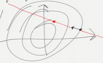
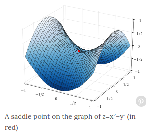
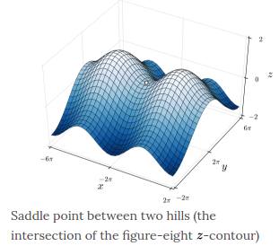
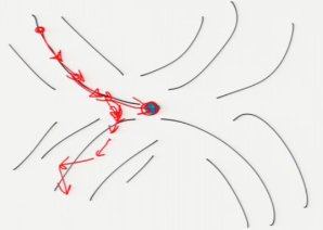
Why GD can not used in saddle?
[Neural nets are unconstrained optimization problems with many, many local minima. They sometimes benefit from the more sophisticated optimization algorithms, but when the input data set is very large, researchers often favor the dumb, blind, stochastic versions of gradient descent.]
[If you're optimizing over a d-dimensional space, the Hessian matrix is a d-by-d matrix and it's usually dense, so most methods that use the Hessian are computationally infeasible when d is large.]
Constrained Optimization (smooth equality constraints)
Goal: Find w that minimizes (maximizes) f(w) subject to g(w) = 0 [<- observe that this is an isosurface]
where g is a smooth fn (may be vector, encoding multiple constraints)
Alg: Use Lagrange_multipliers.
Linear Program
Linear objective fn + linear inequality constraints.
Goal: Find w that maximizes (or minimizes) c . w subject to A w <= b
where A is n-by-d matrix, b in R^n, expressing n linear_constraints: A_i w <= b_i, i in [1, n]
              |    /        \            /
^           --+---O----------\----------/-------  <-- active constraint
 \            |  /.optimum....\        /
  \ c         | /..............\      /
   \          |/................\    /
    \         /.....feasible.....\  /
     \       /|......region.......\/
            / |.................../\
           /  |................../  \
         -/---+-----------------/----\----
         /    |                /      \
        /
       /  <-- active constraint
The set of points that satisfy all constraints is a convex polytope called the feasible_region F. The optimum is the point in F that is furthest in the direction c. [What does convex mean?] A point set P is convex if for every p, q in P, the line segment with endpoints p, q lies entirely in P.
[A polytope is just a polyhedron, generalized to higher dimensions.]
We can always find a global optimum that is a vertex of the polytope.
The optimum achieves equality for some constraints (but not most), called the active_constraints of the optimum.
[In the figure above, there are two active constraints. In an SVM, active constraints correspond to the samples that touch or violate the slab.]
[Sometimes, there is more than one optimal point. For example, in the figure above, if c pointed straight up, every point on the top horizontal edge would be optimal. The set of optimal points is always convex.]
Example: EVERY feasible_point (w, alpha) gives a linear classifier:
----------------------------------------------------------------
| Find w, alpha that maximizes 0                               |
| subject to y_i (w . X_i + alpha) >= 1    for all i in [1, n] |
----------------------------------------------------------------
IMPORTANT:
The data are linearly separable iff the feasible region is not the empty set.
        ^
        |----- Also true for maximum margin classifier (quadratic program)
Algs for linear programming:
- Simplex (George Dantzig, 1947) [Indisputibly one of the most important algorithms of the 20th century.] [Walks along edges of polytope from vertex to vertex until it finds optimum.]
- Interior point methods
[Linear programming is very different from unconstrained optimization; it has a much more combinatorial flavor. If you knew which constraints would be the active constraints once you found the solution, it would be easy; the hard part is figuring out which constraints should be the active ones. There are exponentially many possibilities, so you can't afford to try them all. So linear programming algorithms tend to have a very discrete, computer science feeling to them, like graph algorithms, whereas unconstrained optimization algorithms tend to have a continuous, numerical optimization feeling.]
[Linear programs crop up everywhere in engineering and science, but they're usually in disguise. An extremely useful talent you should develop is to recognize when a problem is a linear program.]
[A linear program solver can find a linear classifier, but it can't find the maximum margin classifier. We need something more powerful.]
Quadratic program
Quadratic, convex objective fn + linear inequality constraints.
Goal:  Find w that minimizes f(w) = w^T Q w + c^T w
       subject to A w <= b

       where Q is a symmetric, positive definite matrix.

A matrix is _positive_definite_ if w^T Q w > 0 for all w != 0.
Only one local minimum!
[If Q is indefinite, so f is not convex, then the minimum is not unique and quadratic programming is NP-hard.]
Example: Find maximum margin classifier.
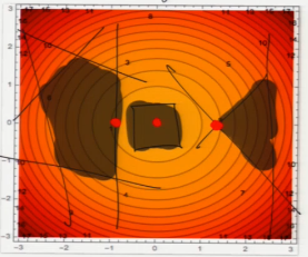 [Show circular contour; draw polygon on top; show constrained minimum.
In an SVM, we are looking for the point in this polygon that's closest to
the origin. Example with one active constraint; example with two.]
[Show circular contour; draw polygon on top; show constrained minimum.
In an SVM, we are looking for the point in this polygon that's closest to
the origin. Example with one active constraint; example with two.]
Algs for quadratic programming:
- Simplex-like
- Sequential minimal optimization (SMO, used in LIBSVM)
- Coordinate descent (used in LIBLINEAR)
[One clever idea used in SMO is that they do a line search that uses the Hessian, but it's cheap to compute because they don't walk in the direction of steepest descent; instead they walk along just one or a few coordinate axes at a time.]
Convex Program (EE 127/227A/227B)
Convex objective fn + convex inequality constraints.
[What I've given you here is, roughly, a sliding scale of optimization problems of increasing complexity, difficulty, and computation time. But even convex programs are relatively easy to solve. When you're trying to address the needs of real-world applications, it's not uncommon to devise an optimization problem with crazy inequalities and an objective function that's nowhere near convex. These are sometimes very, very hard to solve.]