Tensorflow 简单线性回归实例
Table of Contents
1 Tensorflow 2 MNIST实例分析
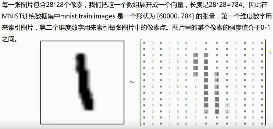
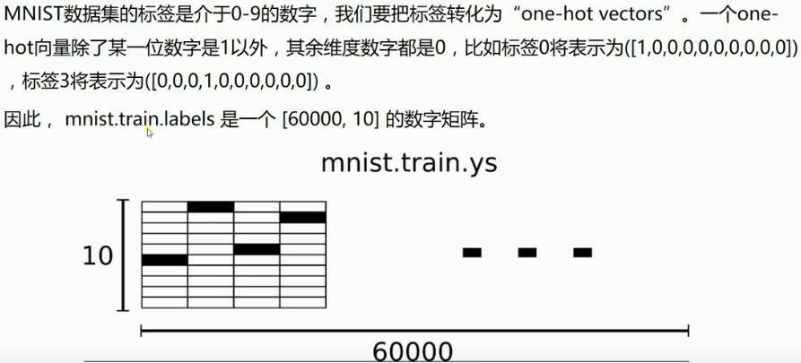
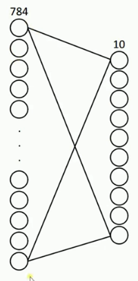
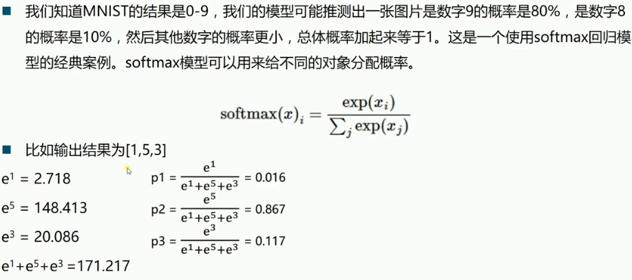
1.0.1 MNIST introduction
2 简单非线性回归实例
<<包导入>>
<<数据准备>>
# numpy构造(with/without noise)
# 从已有数据集导入内存
# 设置批次大小
<<图构造>>
# 一模,两函,两器
<<图计算>>
# 运行两器
# 结果分析
# 绘图

import matplotlib.pyplot as plt
import numpy as np
import tensorflow as tf
# 使用 numpy 生成200个随机点
x_data = np.linspace(-0.5, 0.5, 200)[:, np.newaxis] (Dataset)
noise = np.random.normal(0, 0.02, x_data.shape)
y_data = np.square(x_data) + noise
注意这里构造的是整个数据集 (sample_num, smaple_dimension),有两个原因必须这么做:
- 因为后面要做 one_sample * W + b 的矩阵乘法 所以这里必须给出 sample dimension
- 因为后面喂数据给 placeholder 的时候,是把 run(fetch, feed) 中的feed一行一行拿出来喂进 NN 中
所以他必须是一个二维数组, 注意神经网络是就像一个函数 f(x), 他是针对单个数据点进行预测的. 这点千万搞清楚. 这里和这里是配套使用的,必须要保持一致.
                                    数据集形状                           单个样本形状
                                    ---------------                      ---------
x_data = np.linspace(-0.5, 0.5, 200)[:, np.newaxis]   x = tf.placeholder([None, 1])

                                                  \ /
                                                   +
                                                  / \
                                                 v   v
                       tf.run(train, feed_dict={ x : x_data})
rank=1     rank=2
------     -------
(200, ) vs (200, 1)

In [2]: import numpy as np

In [9]: x_data = np.linspace(-0.5, 5, 200)

In [36]: x_data.shape
Out[42]: (200,)    <====

In [43]: x_data = np.linspace(-0.5, 5, 200)[:, np.newaxis]

In [64]: x_data.shape
Out[68]: (200, 1)  <====
图结构与其在代码中的名称示意图
layer name:        input layer      1-hiden layer      output layer

                      |<--------------->|<--------------->|
                      |   Weights_L1    |   Weights_L2    |
output of
this layer:          'x'              'L1'           'prediction'

                                        *
                                        *
                                        *                              +-- square of residual
                                        *                              |
                      *                 *                 *       <========>      y
                                        *
                                        *
                                        *
                                        *
                                        *
# 定义两个 placeholder
x = tf.placeholder(tf.float32, [None, 1]) (placeholder)
y = tf.placeholder(tf.float32, [None, 1])

# 定义神经网络中间层
Weights_L1 = tf.Variable(tf.random_normal([1, 10]))
biases_L1 = tf.Variable(tf.zeros([1, 10]))
Wx_plus_b_L1 = tf.matmul(x, Weights_L1) + biases_L1
L1 = tf.nn.tanh(Wx_plus_b_L1)

# 定义神经网络输出层
Weights_L2 = tf.Variable(tf.random_normal([10, 1]))
biases_L2 = tf.Variable(tf.zeros([1, 1]))
Wx_plus_b_L2 = tf.matmul(L1, Weights_L2) + biases_L2
prediction = tf.nn.tanh(Wx_plus_b_L2)

# 二次代价函数 -> 优化器 -> 最小化代价函数
loss = tf.reduce_mean(tf.square(y - prediction))
optimizer = tf.train.GradientDescentOptimizer(0.1)
train = optimizer.minimize(loss)
# 初始化器
init = tf.global_variables_initializer()
                         None 表示喂食数据时自动计算
                               -----
x = tf.placeholder(tf.float32, [None, 1])
                               ---------
                         不论以后喂给我的数据点是什么形状,
                         我都将其转换成(~,1)的形状.
with tf.Session() as sess:
    # 运行初始化器
    sess.run(init)
    # 运行优化器
    for _ in range(2000):
        sess.run(train, feed_dict={x: x_data, y: y_data})

    # 获得预测值
    prediction_value = sess.run(prediction, feed_dict={x: x_data})

    # 绘图
    plt.figure()
    plt.scatter(x_data, y_data) (scatter)
    plt.plot(x_data, prediction_value, 'r-', lw=5) (plot)
    plt.show()
线图参数中的 'r-'('r' 红色, '-' 实线), 'lw=5'表示线宽 5 pixel

3 简单MNIST数据集分类
<<包导入>>
<<数据准备>>
# numpy构造(with/without noise)
   # 设置批次大小
# 从已有数据集导入内存
   # 设置批次大小
<<图构造>>
# 一模,两函,两器
<<图计算>>
# 运行两器
# 结果分析
# 绘图
 1: import tensorflow as tf
 2: from tensorflow.examples.tutorials.mnist import input_data
 3:
 4: # 载入数据
 5: mnist = input_data.read_data_sets("MNIST", one_hot=True) (one_hot)
 6:
 7: # 设置批次大小
 8: batch_size = 100 (batch_size)
 9: # 计算共有多少批次
10: n_batch = mnist.train.num_examples // batch_size (floor division)
11:
12: # 定义两个 placeholder
13: x = tf.placeholder(tf.float32, [None, 784])
14: y = tf.placeholder(tf.float32, [None, 10])
15:
16: # 创建简单神经网络(无隐藏层)
17: W = tf.Variable(tf.zeros([784, 10]))
18: b = tf.Variable(tf.zeros([10]))
19: prediction = tf.nn.softmax(tf.matmul(x, W) + b)
20:
21: # 二函,二器
22: init = tf.global_variables_initializer()
23: optimizer = tf.train.GradientDescentOptimizer(0.2)
24: loss = tf.reduce_mean(tf.square(y-prediction))
25: train = optimizer.minimize(loss)
26:
27: # 预测对错存在一个向量中
28: correct_prediction = tf.equal(tf.argmax(y,1), tf.argmax(prediction, 1)) (count correct prediction)
29: # 计算准确率
30: accuracy = tf.reduce_mean(tf.cast(correct_prediction, tf.float32))
31:
32:
33: # 图计算
34: with tf.Session() as sess:
35:     sess.run(init)
36:     # 采取训练一轮就测试一轮的方式
37:     for epoch in range(21):
38:         # 训练模型
39:         acc_train = 0
40:         for batch in range(n_batch):
41:             batch_xs, batch_ys = mnist.train.next_batch(batch_size)
42:             _, acc_train = sess.run([train, accuracy], feed_dict={x:batch_xs, y:batch_ys})
43:
44:         # 测试模型
45:         # 测试集必须使用已经训练完毕的模型
46:         acc_test = sess.run(accuracy, feed_dict={x:mnist.test.images, y:mnist.test.labels})
47:         print("Iter " + str(epoch) + " ,Train:" + str(acc_train) + " ,Test:" + str(acc_test))
48:
数据集label总共有几种取值,就导入成几维的 one_hot 向量. 这里数据集 label 总共有 0~9 共10种取值, 就把每个 label 导入为10维的one_hot向量.
batch 是以一个矩阵的形式(batch_size * smaple_dimension)喂食数据
'correct_prediction'中存储的是 boolean 值
y 中存有60000个one-hot vector:(60000, 10), 每个针对y的第二维度(也就是'行',每个
sample)做 argmax, 可以得到 60000 个 max_value_index 组成的一个 Tensor; 同样的
prediction经过argmax也会得到60000个 max_value_index 组成的一个 Tensor. 然后对
这两个 Tensor 进行 element-wise 比较就可以得到一个 (60000,1) 的boolean Tensor.


            one_hot vector of                                                        prediction(output
             label of                                                                of NN) of
index        one sample                                                               one sample

  0              0  \                                                                  /  0.01
  1              0   |                                                                |   0.12
  2              0   |                                                                |   0.07
  3              0   |                          equal or not                          |   0.01
  4              1   | index of max value = 4   ============= 5 = index of max value  |   0.02
  5              0   |                                |                               |   0.7
  6              0   |                                |                               |   0.01
  7              0   |                                |                               |   0.03
  8              0   |                                |                               |   0.15
  9              0  /                                 v                                \  0.15
                                                 equal => True
                                             not equal => False
                ------------------------>---------------------|
                | tf.equal                                    |                tf.reduce_mean
                |                                             |              -----------------> correct
    +---------------------+                                   v              ^                  accuracy
    |                     |                                   |              |
tf.argmax             tf.argmax
+----------           +-----------------------------
|0001000000           |.7 .2 .1 .0 .0 .0 .0 .0 .0 .0          t             1.0
+----------           +-----------------------------
 0001000000            .7 .2 .1 .0 .0 .0 .0 .0 .0 .0          f             0.0
 0001000000            .7 .2 .1 .0 .0 .0 .0 .0 .0 .0          t             1.0
 0001000000            .7 .2 .1 .0 .0 .0 .0 .0 .0 .0          t             1.0
 ...                   ...                                    .              .
 ...                   ...                                    .              .
 ...                   ...                                    .              .
 0001000000            .7 .2 .1 .0 .0 .0 .0 .0 .0 .0          f             0.0

                                                              |              |
                                                              v              ^
                                                              | tf.cast      |
                                                              -------->------|
3.1 cross_entropy
\(\theta(s)=\frac{1}{1+e^{-s}}\)
\(loss(f)=1/N\sum_{n=1}^N\theta(-y_nw^T_tx_n)(-y_nx_n)\)
tf.reduce_mean(tf.sigmoid(tf.negative(tf.multiply(y, prediction))))