Tensorflow 实现卷积神经网络
Table of Contents
1 Tensorflow-CNN
CNN: 局部感受和权值共享
卷积核可以理解成一个模式匹配或者更形象一点,理解成滤波器.
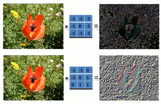
有几个卷积核就可以采样出几个特征图.
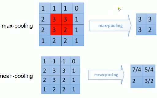
池化上接卷积层, 一般有三种: max-pooling, mean-pooling, random-pooling
padding
same padding: 不保证; 可以超过图片边界采样
valid padding: 不保证; 不可以超过
一张 2*3 的图片,经过 "SAME" 和 "VALID" 两种方式采样, 会得到的不同结果

+---+---+---+
|   |   |   |
|---+---+---|
|   |   |   |
+---+---+---+

以 2*2 步长为 2 的窗口以 same padding 的方式进行 pooling 操作

...........                ............
.---------.--+      +---+--.-+---+****.
.|   |   |.  |      |   |  . |   |   *.
.|---+---+.--| ---> |---+--.-+---|****. ---- 因为不够 2*2 了所以这里会
.|   |   |.  |      |   |  . |   |   *.      多补出一列, 最终会采样出
.---------.--+      +---+--.-+---+****.      1*2 的矩阵
..........                 ............


以 2*2 步长为 2 的窗口以 valid padding 的方式进行 pooling 操作

...........
.---------.--+      +---+---+---+
.|   |   |.  |      |   |   |   |
.|---+---+.--| ---> |---+---+---+       ---- 不够了就停止
.|   |   |.  |      |   |   |   |            最终会采样出
.---------.--+      +---+---+---+            1*1 的矩阵
..........
2 CNN 应用于MNIST数据集分类
<<包导入>>
# <<导入 projector: for embeddings 可视化>>


<<数据准备>>
# numpy构造(with/without noise)
# 数据集导入内存(one_hot or not)
# 截取已经存在数据集

<<图参数>>
# 批次大小
# 批次数量
# dropout 保留率
# 数据集位置

<<工具函数与工具声明>>
# 对某些 Variable 进行 OP 并 summary
# <<def Variable: for embeddings 可视化>> as untrainable Variable, stack front 3000 img, give name 'embeddings'
# <<file IO: for embeddings 可视化>> read in one_hot labels, argmax get true labels, write to file in one-label-one-line format
# W, b 初始化工具函数

<<图构造>>
# 一神: NN layers, name_scope for TB, 参数 summary
# 1. placeholders
#    1.1 x: dataset placeholder,
#    + <<def OP: for img process, CNN >> reshape x                             ------+
#    1.2 y: labelset placeholder,                                                    |
#    1.3 keep_prob: dropout, keep rate of certain layer's nodes                      |
# 2. Variables                                                                       |
#    2.0 名称空间设置                                                                |
#    2.1 第一层权重 W, 声明 summary tf.summary.scalar/image/histogram node           |
#    2.2 第一层偏置 b, 声明 summary tf.summary.scalar/image/histogram node           |
#    + <<conv2d layer: for CNN>> 只接受 [batch_size, height, width, channels] 格式 <-+
#    + <<max_pool layer: for CNN>>

# 3. Operations
#    3.1 第一层输出(active_fn(score)), 声明 summary tf.summary.scalar/image/histogram node

# 两函:
#   1. err_fn:
#      1.1 名称空间设置
#      1.2 err fn(单点错误), 声明 summary, tf.summary.scalar/image/histogram node
#   2. loss_fn:
#      2.1 名称空间设置
#      2.2 loss fn(整体错误), 声明 summary, tf.summary.scalar/image/histogram node

# 两器:
#   1. 初始化器
#   2. 优化器
#      2.1 名称空间设置

# 准确率计算
#   1. correct_prediction
#      1.1 名称空间设置
#   2. accuracy
#      2.1 名称空间设置

# 合并summary

# 配置 embeddings 可视化参数

<<图计算>>
# 运行初始化器
# summary Writer for TB
# for epoch_num: <<
#          1. for batch_num:
#                 1.1 x_y_of_next_batch;
#                 1.2 运行 优化器计算 and summary计算
#          2. 运行准确率计算
# matplot绘图
卷积核: [shape, image_channel, 卷积核个数], 就是缩减版的权重. 局部感受和权值共享.
import tensorflow as tf
from tensorflow.examples.tutorials.mnist import input_data

mnist = input_data.read_data_sets('MNIST', one_hot=True)

batch_size = 100

n_batch = mnist.train.num_examples // batch_size

# 初始化权值和截距
def weight_variable(shape):
    """
    shape = [filter_height, filter_width, in_channels, number]
    """
    initial = tf.truncated_normal(shape, stddev=0.1)
    return tf.Variable(initial)

def bias_variable(shape):
    initial = tf.constant(0.1, shape=shape)
    return tf.Variable(initial)

# 卷基层
def conv2d(x, W):
    """
    x input tensor of shape `[batch, in_height, in_width, in_channels]`

                                                                                 卷积核个数
                                                                                 ------------
    W filter / kernel tensor of shape [filter_height, filter_width, in_channels, out_channels]

    strides [1, x, y, 1]
    `strides[0]=strides[3]=1` strides[1] 代表x方向的步长, strides[2]代表y方向的步长

    padding: a `string` from: `"SAME" or "VALID"`,
    """
    return tf.nn.conv2d(x, W, strides=[1,1,1,1], padding='SAME')

# 池化层
def max_pool_2x2(x):
    """
    ksize [1, x, y, 1] 窗口大小 ksize[1] 表示x方向的大小, ksize[2]表示y方向的大小

    strides [1, x, y, 1]
    `strides[0]=strides[3]=1` strides[1] 代表x方向的步长, strides[2]代表y方向的步长
    """
    return tf.nn.max_pool(x, ksize=[1,2,2,1], strides=[1,2,2,1], padding='SAME')

# 卷积核与池化矩阵的移动都是通过设置 strides 来指定的,且格式固定 [1, x, y, 1]
# 不同的是两者大小的设定, 卷积核通过 filter 来设置[filter_height, filter_width, in_channels, out_channels]
# 池化矩阵大小通过 ksize 来设置[1, x, y, 1]

# 定义两个placeholder
x=tf.placeholder(tf.float32, [None, 784])
y=tf.placeholder(tf.float32, [None, 10])

# 改变x的格式为4D向量[batch, in_height, in_width, in_channels]
x_image = tf.reshape(x, [-1, 28, 28, 1])

# 初始化第一个卷基层的权值和偏置
W_conv1 = weight_variable([5,5,1,32]) #5*5的采样窗口, 32个卷积核从1个平面抽取特征
b_conv1 = bias_variable([32]) # 每一个卷积核一个偏置

# 把x_image和权值向量进行卷积, 再加上偏置值, 然后应用于 relu 激活函数
h_conv1 = tf.nn.relu(conv2d(x_image, W_conv1) + b_conv1)
h_pool1= max_pool_2x2(h_conv1) #进行max-pooling

# 初始化第二个卷基层的权值和偏置
W_conv2 = weight_variable([5,5,32,64]) #5*5的采样窗口, 64个卷积核从32个平面抽取特征
b_conv2 = bias_variable([64]) # 每一个卷积核一个偏置

# 把h_pool1和权值向量进行卷积, 再加上偏置值, 然后应用于 relu 激活函数
h_conv2 = tf.nn.relu(conv2d(h_pool1, W_conv2) + b_conv2)
h_pool2= max_pool_2x2(h_conv2) #进行max-pooling

# 28*28的图片第一次卷积后还是28*28, 第一次池化之后变为14*14
# 第二次卷积后为14*14, 第二次池化后变为7*7
# 经过上面操作后得到 64 张 7*7 的 feature map

# 初始化第一个全连接层的权值
W_fc1 = weight_variable([7*7*64, 1024]) # 上一层有 7*7*64 个神经元, 全连接层有2014神经元
b_fc1 = bias_variable([1024])

# 把池化层2的输出扁平化为1维
h_pool2_flat = tf.reshape(h_pool2, [-1, 7*7*64])
# 求第一个全连接层的输出
h_fc1= tf.nn.relu(tf.matmul(h_pool2_flat, W_fc1) + b_fc1)

# keep_prob 用来表示神经元的 dropout keep 率
keep_prob = tf.placeholder(tf.float32)
h_fc1_drop = tf.nn.dropout(h_fc1, keep_prob)

# 初始化第二个全连接层
W_fc2 = weight_variable([1024, 10]) # 上一层有 7*7*64 个神经元, 全连接层有2014神经元
b_fc2 = bias_variable([10])

# 计算输出
prediction = tf.nn.softmax(tf.matmul(h_fc1_drop, W_fc2) + b_fc2)

# 交叉熵代价函数
cross_entropy = tf.reduce_mean(tf.nn.softmax_cross_entropy_with_logits_v2(labels=y, logits=prediction))
# 使用 AdamOptimizer 优化
train_step = tf.train.AdamOptimizer(1e-4).minimize(cross_entropy)
# 结果存放在一个bool list 中
correct_prediction = tf.equal(tf.argmax(prediction, 1), tf.argmax(y, 1))
# 求准确率
accuracy = tf.reduce_mean(tf.cast(correct_prediction, tf.float32))


# 图计算
with tf.Session() as sess:
    sess.run(tf.global_variables_initializer())
    for epoch in range(21):
        for batch in range(n_batch):
            batch_xs, batch_ys = mnist.train.next_batch(batch_size)
            sess.run(train_step, feed_dict={x:batch_xs, y:batch_ys, keep_prob:0.7})

        acc = sess.run(accuracy, feed_dict={x:mnist.test.images, y:mnist.test.labels, keep_prob:1.0})
        print("Iter " + str(epoch) + ", Testing Accuracy= " + str(acc))
0 - c77968f5-e34e-486e-b388-69e1e8d4cca8
这里可通过 FileWriter 写入两次文件, 分别写入 train_accu 的 summary 和 test_accu 的 summary, 这样在 tensorboard 中就可以同时看到两条 accuracy 变化曲线.通过这种方式, 可以很方便的判断模型是否存在 overfitting 的情况.