Tensorflow Debug 介绍
Table of Contents
1 介绍 tensorflow debuger
1.1 tfdbg CLI 界面介绍
想使用 tfdbg 的 CLI 模式, 只需两步:
- wrap sess with
debug.LocalCLIDebugWrapperSession - 运行源码时, 给 command 加入
--debugflag
from tensorflow.python import debug as tf_debug
sess = tf_debug.LocalCLIDebugWrapperSession(sess)
tfdbg CLI 界面
--- run-start: run #1: 1 fetch (accuracy/accuracy/Mean:0); 2 feeds -------------
| <-- --> | run_info
| run | invoke_stepper | exit |
                                                                                             UP
TTTTTT FFFF DDD  BBBB   GGG
  TT   F    D  D B   B G
  TT   FFF  D  D BBBB  G  GG
  TT   F    D  D B   B G   G
  TT   F    DDD  BBBB   GGG

======================================
Session.run() call #1:

Fetch(es):
  accuracy/accuracy/Mean:0

Feed dict:
  input/x-input:0
  input/y-input:0
======================================

Select one of the following commands to proceed ---->
  run:
    Execute the run() call with debug tensor-watching
  run -n:
    Execute the run() call without debug tensor-watching
  run -t <T>:
    Execute run() calls (T - 1) times without debugging, then execute run() once more with deDN
--- Scroll (PgDn): 0.00% --------------------------------------------------------- Mouse: ON --
tfdbg>
1.2 tfdbg TensorBoard 界面介绍
import numpy as np
import tensorflow as tf

# Truth values for the linear model.
k_true = [[1, -1], [3, -3], [2, -2]]
b_true = [-5, 5]
num_examples = 128

with tf.Session() as sess:
    # Input place holders.
    x = tf.placeholder(tf.float32, shape=[None, 3], name="x")
    y = tf.placeholder(tf.float32, shape=[None, 2], name="y")

    # Deine model architecture, loss and training operator.
    dense_layer = tf.keras.layers.Dense(2, use_bias=True)
    y_hat = dense_layer(x)
    loss = tf.reduce_mean(
        tf.keras.losses.mean_squared_error(y, y_hat), name="loss")
    train_op = tf.train.GradientDescentOptimizer(0.05).minimize(loss)

    # Initializer model variables.
    sess.run(tf.global_variables_initializer())
    # Saver
    saver = tf.train.Saver()

    for i in range(50):
        # Generate synthetic training data.
        xs = np.random.randn(num_examples, 3)
        ys = np.matmul(xs, k_true) + b_true

        save_path = saver.save(sess, '/tmp/logdir/lin_dbg.ckpt')

        loss_val, _ = sess.run([loss, train_op], feed_dict={x: xs, y: ys})
        print("Iter %d: loss = %g" % (i, loss_val))
import numpy as np
import tensorflow as tf
from tensorflow.python import debug as tf_debug

# Truth values for the linear model.
k_true = [[1, -1], [3, -3], [2, -2]]
b_true = [-5, 5]
num_examples = 128

# Input place holders.
x = tf.placeholder(tf.float32, shape=[None, 3], name="x")
y = tf.placeholder(tf.float32, shape=[None, 2], name="y")

# Deine model architecture, loss and training operator.
dense_layer = tf.keras.layers.Dense(2, use_bias=True)
y_hat = dense_layer(x)
loss = tf.reduce_mean(
    tf.keras.losses.mean_squared_error(y, y_hat), name="loss")
train_op = tf.train.GradientDescentOptimizer(0.05).minimize(loss)

# Init OP
init_op = tf.global_variables_initializer()

# Saver
# saver = tf.train.Saver()

with tf.Session() as sess:
    # Initializer model variables.
    sess.run(init_op)

    # sess = tf_debug.TensorBoardDebugWrapperSession(sess, "yiddiEdge:7000")

    for i in range(50):
        # Generate synthetic training data.
        xs = np.random.randn(num_examples, 3)
        ys = np.matmul(xs, k_true) + b_true

        # save_path = saver.save(sess, '/tmp/logdir/lin_dbg.ckpt')

        loss_val, _ = sess.run([loss, train_op], feed_dict={x: xs, y: ys})
        print("Iter %d: loss = %g" % (i, loss_val))
0 - 0eac0512-9001-40a5-aff7-d50b30dfa1a8
想使用 tfdbg 并对其进行可视化, 注意严格按照如下步骤来,
- run un-modified python code to produce
.ckptfile - execute TB command without –debug flag
- modify python code, import debug and wrap sess, TB still run now.
- run modified python code
如果, 完全关闭 TB 之后再修改代码, 会 lead an rpc error.
_Rendezvous: <_Rendezvous of RPC that terminated with (StatusCode.UNAVAILABLE, Connect Failed)>
需要在 tensorboard 命令行中加入如下参数
debugger_port:(require 'ob-async)
ob-async
tensorboard --logdir /tmp/logdir --debugger_port 7000源码中导入 tensorflow.python.debug
# To connect to the debugger from your tf.Session:
from tensorflow.python import debug as tf_debug
- wrap
sesswithdebug.TensorBoardDebugWrapperSession(sess, "local_URL")
sess = tf.Session()
sess = tf_debug.TensorBoardDebugWrapperSession(sess, "yiddiEdge:7000")
sess.run(my_fetches)

# To connect to the debugger using hooks, e.g., from tf.Estimator:
from tensorflow.python import debug as tf_debug
hook = tf_debug.TensorBoardDebugHook("yiddiEdge:7000")
my_estimator.fit(x=x_data, y=y_data, steps=1000, monitors=[hook])
1.3 其他处理部分
<<get-pid>>
<<kill-pid>>
<<del-graph-summary>>
<<tensorboard-run>>
<<run-tensorboard>>
ps -aux | grep "python" | grep -E "(default|tfdbg|tensorboard)" | grep -v "grep" | awk '{print $2}'
14526
;; 取元素
(defun r1l(tbl)
  (mapcar (lambda (x) (number-to-string (car x))) tbl)
  )
;; (print pid)
;; (print (reduce-one-layer pid))
(mapcar #'shell-command-to-string
        (mapcar (lambda (x) (concat "kill " x)) (r1l pid))))
rm -rf /tmp/logdir/*
ls /tmp/logdir
1.3.1 TB debugger 界面介绍
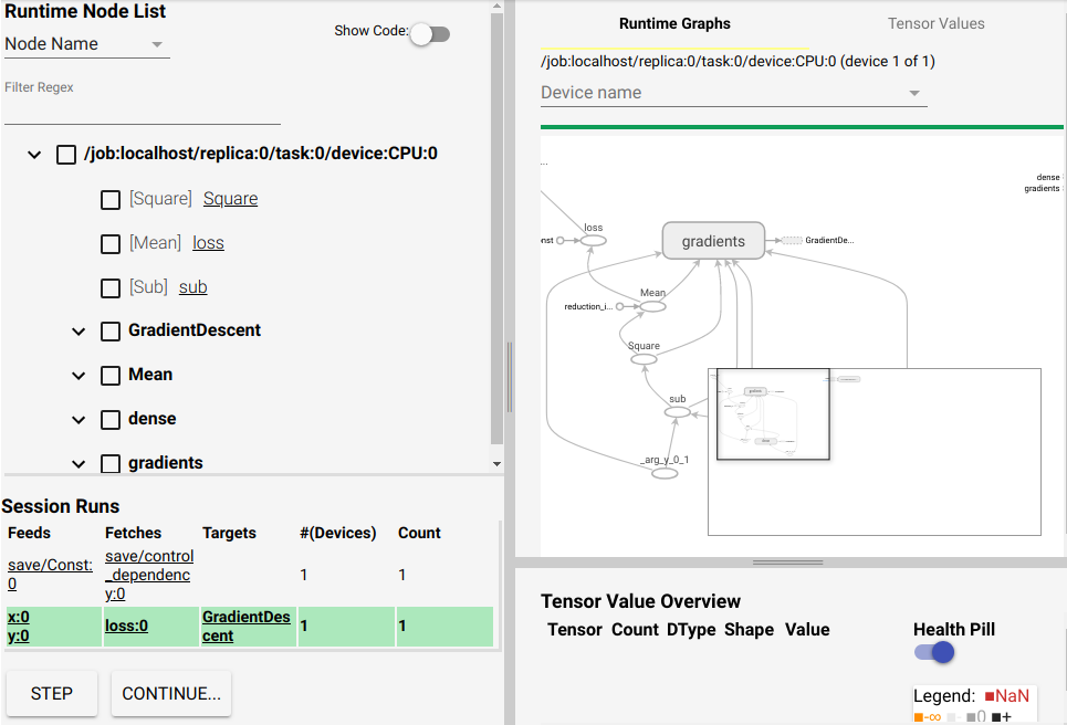
界面大概可以分成4块, 左上角是树型结构是根据模型的 name_scope 绘制. 其中 gradients 节点是 BP 算法的重要部分, 应该多加关注. 他基本决定了你的 model 是如何一步一步训练的.
右上角就是我们熟悉的 graph 对应的结构图, 其中每一个 node 右键都可以点击 continue to. 这样他就会出现在右下角的列表中, 这个列表用于显示 Tensor Value.
你当然也可以让 gradient node continue, 右下角的最后一列是一个黑白色的条, 将鼠标悬停其上可以查看每个 node 的各种信息,
- mean value of elements in this tensor
- stddev value of elements in this tensor
- max value of elements in this tensor
- # of elements
- # of +
- # of -
当你点击 "click to view", 你会发现这个 Tensor 的详细视图, 你可以使用 numpy slicing 的方式去界定查看范围.
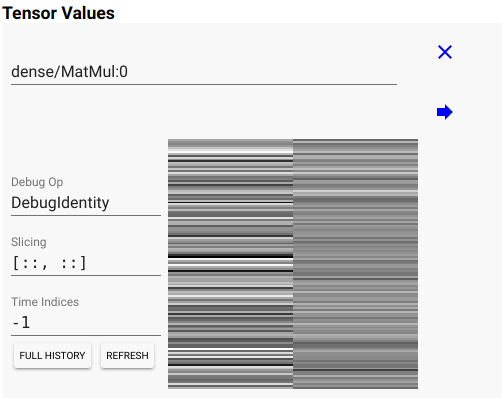
当你设置 [::, 0] 表示我要查看该 Tensor 的第0列随优化次数的变化
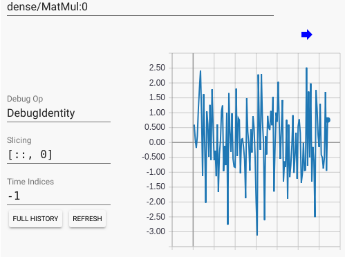
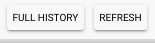
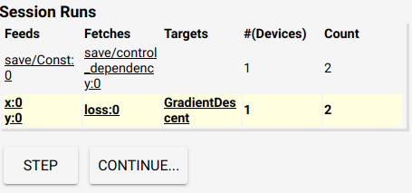
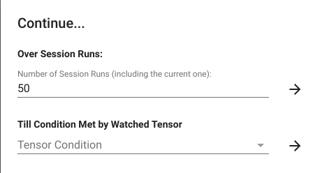
我们还可以看看 loss Tensor, 他是一个数值, 当我们打开他的 "click to view", 然后点击 "FULL HISTROY" 按键, 然后点击左下角的 "CONTINUE", 然后在弹出的界面中输入 "50" 次, 可以看到他随优化次数而产生的变化, 这个变化是动态的, 整个界面的所有数值都会随之改变, 你可以观察到 loss 曲线的变化, 可以看到随着模型的训练, 这个 loss 值是如何变化的.
1.4 一个 broken 例子
python -m tensorflow.python.debug.examples.debug_mnist
这会从官网下在数据集, 和一段有bug的源码, 训练之后可以看到第二行出现了精度上升, 紧接着急剧下降, 然后一直维持在 0.098. 这种情况在训练 NN 时非常常见, 一般都是因为模型中出现了 "bad numerical values", 像是 inf or non. 我们下面要做的就是找到哪个 Tensor 出了问题.
Accuracy at step 0: 0.1113
Accuracy at step 1: 0.2883  <===
Accuracy at step 2: 0.098
Accuracy at step 3: 0.098
Accuracy at step 4: 0.098
Accuracy at step 5: 0.098
Accuracy at step 6: 0.098
Accuracy at step 7: 0.098
Accuracy at step 8: 0.098
Accuracy at step 9: 0.098
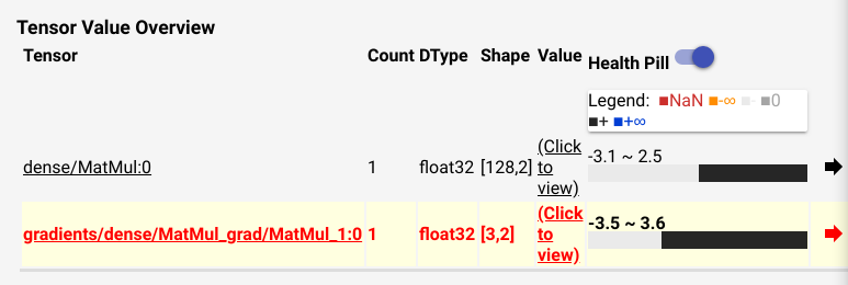
我们可以在这一步的 "Till condition met by watched tensor", 从下拉选框中选择 "contains +/- or NaN", 这样模型的训练会忽略次数("50"), 一直训练直到某个 node 出现了 inf or nan 值, 这时候会停下, 并显示那个节点为红色.

我们可以点开 click to view, 其中显示的橙色线条就代表 inf or nan 值.
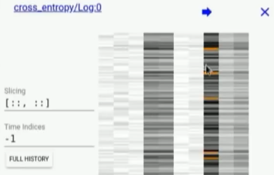
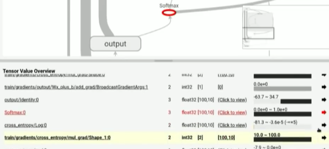
但是, 为什么 inf or nan 会出现在 cross_entropy 节点中呢.
- 查看源代码中 cross_entropy 节点的定义, 主要看该节点的输入节点
- 从右上角的 graph 结构图中查其输入节点, 这里 cross_entropy 输入节点为 softmax, 右键 -> expand and heighlight 这样在 Tensor value overview(右下角) 部分 我们就可以看到被高亮的 softmax 此时的值. 很明显这里 softmax 为 0. 但我们对 softmax 取 log 求cross_entropy的时候就会产生 inf.